Eigil Fjeldgren Rischel [index]
Eigil Fjeldgren Rischel [index]
My name is Eigil Fjeldgren Rischel. I'm a a Research Consultant at the Tallinn University of Technology, in the Laboratory for Compositional Systems and Methods. I'm currently employed working on the Safeguarded AI project.
Before that, I completed a PhD in Computer and Information Sciences at the University of Strathclyde. Neil Ghani, Jules Hedges, and Radu Mardare all served as my advisors at various times.
I mainly work on applications of category theory to probability and statistics. I am particularly interested in synthetic methods - that is, methods which abstract from particular models of probability to capture the essential features that allow us to reason about random processes. Much of my research has centered around the notion of Markov Categories. Markov Fibrations › Preliminaries › Markov categories
This website is a "forest", made with the forester tool. It contains various notes I've made over the years, as well as some more structured blog posts.
Click on the headings below to expand, or on the bracketed link next to them to go to the relevant page.
List of Publications [efr-0032]
List of Publications [efr-0032]
Reference Metric Equational Theories [mardare-ghani-rischel-2025]
- September 17, 2025
-
Radu Mardare, Neil Ghani, Eigil Fjeldgren Rischel
-
10.4204/eptcs.428.11
Reference Metric Equational Theories [mardare-ghani-rischel-2025]
- September 17, 2025
- Radu Mardare, Neil Ghani, Eigil Fjeldgren Rischel
- 10.4204/eptcs.428.11
Abstract
- September 17, 2025
-
Radu Mardare, Neil Ghani, Eigil Fjeldgren Rischel
Abstract
- September 17, 2025
- Radu Mardare, Neil Ghani, Eigil Fjeldgren Rischel
This paper proposes appropriate sound and complete proof systems for algebraic structures over metric spaces by combining the development of Quantitative Equational Theories (QET) with the Enriched Lawvere Theories. We extend QETs to Metric Equational Theories (METs) where operations no longer have finite sets as arities (as in QETs and the general theory of universal algebras), but arities are now drawn from countable metric spaces. This extension is inspired by the theory of Enriched Lawvere Theories, which suggests that the arities of operations should be the lambda-presentable objects of the underlying lambda-accessible category. In this setting, the validity of terms in METs can no longer be guaranteed independently of the validity of equations, as is the case with QET. We solve this problem, and adapt the sound and complete proof system for QETs to these more general METs, taking advantage of the specific structure of metric spaces.
@article{Mardare2025,
  title = {Metric Equational Theories},
  volume = {428},
  ISSN = {2075-2180},
  url = {http://dx.doi.org/10.4204/EPTCS.428.11},
  DOI = {10.4204/eptcs.428.11},
  journal = {Electronic Proceedings in Theoretical Computer Science},
  publisher = {Open Publishing Association},
  author = {Mardare,  Radu and Ghani,  Neil and Rischel,  Eigil},
  year = {2025},
  month = sep,
  pages = {144–160}
}
Reference Convex Duality Made Difficult [rischel-cvxdual-2025]
Reference Convex Duality Made Difficult [rischel-cvxdual-2025]
Convex Duality made Difficult [lcc-001Z]
- April 30, 2024
-
Eigil Fjeldgren Rischel
Convex Duality made Difficult [lcc-001Z]
- April 30, 2024
- Eigil Fjeldgren Rischel
Introduction
- April 30, 2024
-
Eigil Fjeldgren Rischel
Introduction
- April 30, 2024
- Eigil Fjeldgren Rischel
The study of convex functions - in particular, of their optimization (really minimization) is one of the most important fields of applied mathematics. Convexity seems to be one of those incredibly well-chosen hypotheses which is just specific enough to admit a wealth of theorems, just general enough to produce a nontrivial theory (and a large amount of important examples).
Convex optimization, possibly because it has an "analytical" rather than "algebraic" feel, has not been very thoroughly studied by applied category theorists. The one notable exception is Reference [hanks-etal-convex-2024], which studies the decomposition of optimization problems by categorical means. This paper takes a different approach, attempting to define a category with optimization problems as the objects, and to derive theorems about optimization by categorical means.
Convex optimization
- April 30, 2024
-
Eigil Fjeldgren Rischel
Convex optimization
- April 30, 2024
- Eigil Fjeldgren Rischel
Definition Standard form convex optimization problem [lcc-001G]
- April 22, 2024
-
Eigil Fjeldgren Rischel
Definition Standard form convex optimization problem [lcc-001G]
- April 22, 2024
- Eigil Fjeldgren Rischel
A convex optimization problem in standard form consists of
- A convex function f_0: \mathbb {R}^k \to \mathbb {R}
- A list of convex functions f_1, \dots f_n: \mathbb {R}^k \to \mathbb {R}
- A list of affine functions g_1,\dots g_m: \mathbb {R}^k \to \mathbb {R}
Definition Lagrangian of an optimization problem [lcc-002K]
- May 17, 2024
-
Eigil Fjeldgren Rischel
Definition Lagrangian of an optimization problem [lcc-002K]
- May 17, 2024
- Eigil Fjeldgren Rischel
Let f_0: \mathbb {R}^k \to \mathbb {R}, f_1, \dots f_n, g_1 , \dots g_m be a standard-form convex optimization problem, as in Definition [lcc-001G]. Then the Lagrangian of this problem is the function L: \mathbb {R}^k \times \mathbb {R}^n_+ \times \mathbb {R}^m \to \mathbb {R} defined by L(x;\lambda ,\nu ) = f_0(x) + \sum _i \lambda _i f_i(x) + \sum _i \nu _i g_i(x). Recall that \mathbb {R}_+ denotes the nonnegative reals.
Observe that \sup _{\lambda ,\nu } L(x,\lambda ,\nu ) is f_0(x) if x satisfies the constraints of the problem, and \infty otherwise. Hence we can think of this minimization problem as playing a zero-sum game: we choose x, our adversary chooses \lambda ,\nu , and our loss function is L.
It is natural to ask about the existence of Nash equilibria in this game - observe that the existence of an equilibrium (x^*,\lambda ^*,\nu ^*) means that \inf _x \sup _{\lambda ,\nu } L(x,\lambda ,\nu ) = \sup _{\lambda ,\nu } \inf _x L(x,\lambda ,\nu ) = L(x^*,\lambda ^*,\nu ^*). This is of great utility in solving the original problem.
The dual problem is the problem of maximizing the function \inf _x L(x,\lambda ,\nu ). This is always a concave problem.
In the world of convex optimization, two problems whose constraints carve out the same subset of \mathbb {R}^k (and where the function to optimize is the same) would be called equivalent. But they can clearly not be regarded as isomorphic, because the choice of constraint functions makes an important difference to the theory of optimization (for example, it can lead to different dual problems). Here we take the viewpoint that the Lagrangian is really the fundamental object in convex optimization - by passing to a suitable category of Lagrangians, we can make the dual problem into an actual self-duality on this category.
Convex spaces
- April 30, 2024
-
Eigil Fjeldgren Rischel
Convex spaces
- April 30, 2024
- Eigil Fjeldgren Rischel
Definition Convex Space [lcc-0020]
- April 30, 2024
-
Eigil Fjeldgren Rischel
Definition Convex Space [lcc-0020]
- April 30, 2024
- Eigil Fjeldgren Rischel
The category of convex spaces is the category of algebras for the monad \Delta : \mathsf {Set} \to \mathsf {Set} of discrete finite-support distributions. The morphisms are called \Delta -homomorphisms or homomorphisms of convex spaces.
So as not to multiply notation unnecessarily, we simply denote the category of convex spaces by \mathsf {Set}^\Delta , using the usual notation for the Eilenberg-Moore category.
Definition [lcc-002N]
- May 20, 2024
-
Eigil Fjeldgren Rischel
Definition [lcc-002N]
- May 20, 2024
- Eigil Fjeldgren Rischel
A function between vector spaces is called affine if it preserves those linear combinations \sum _i \lambda _i x_i where \sum _i \lambda _i = 1
Definition [lcc-002M]
- May 20, 2024
-
Eigil Fjeldgren Rischel
Definition [lcc-002M]
- May 20, 2024
- Eigil Fjeldgren Rischel
Let X be a convex space. A convex function on X is a function f: X \to \mathbb {R} so that f(\theta x + (1-\theta )x') \leq \theta f(x) + (1-\theta )f(x')
A concave function is a function so that -f is convex (in other words, f satisfies the opposite inequality).
The term "convex function" in this sense clashes with the usual practice of naming structure-preserving functions after the structure they preserve (since convex functions do not preserve the convex structure). Unfortunately this usage is far too established to alter. (Convex functions are called convex because they are exactly those functions where the area above their graph is a convex subset of X \times \mathbb {R}. Although there appears to be no particular reason why the terms convex and concave should not be interchanged, other than convention).
Jensen's Inequality [lcc-002R]
- May 19, 2024
-
Eigil Fjeldgren Rischel
Jensen's Inequality [lcc-002R]
- May 19, 2024
- Eigil Fjeldgren Rischel
The inequality f(\theta x + (1-\theta )x') \leq \theta f(x) + (1-\theta )f(x'), which holds whenever f is convex, is called Jensen's inequality. Sometimes this name is used for a stronger version of this inequality, like the claim that f(\mathbb {E} X) \leq \mathbb {E} f(X) if X is a random variable valued in the domain of f. These generally follow just from convexity of f.
[lcc-002Q]
- May 19, 2024
-
Eigil Fjeldgren Rischel
[lcc-002Q]
- May 19, 2024
- Eigil Fjeldgren Rischel
There is an natural way to extend the convex structure of \mathbb {R} to both \lsqb -\infty , \infty \rpar and \lpar -\infty , \infty \rsqb , by the convention that any nontrivial convex combination involving an infinity is equal to that infinity. This also gives the adjectives convex and concave a meaning when applied to functions X \to \lpar -\infty , \infty \rsqb . For example, a function f: X \to \lpar -\infty , \infty \rsqb is convex if and only if the subset where it's finite is a convex subset of X, and it's a convex function in the ordinary sense on this set.
This doesn't work for the extended real line \eRR = \lsqb -\infty , \infty \rsqb , since there is no sensible interpretation of \theta \cdot -\infty + (1-\theta )\infty . We will inescapably meet some functions which take value in the full extended reals, but where we still wish to speak of their convexity (or concavity).
Hence we adopt the convention that a function f: X \to \eRR is convex if it obeys Jensen's inequality whenever it makes sense, i.e whenever we do not have f(x) = -\infty , f(x') = \infty or vice versa.
Proposition [lcc-002O]
- May 20, 2024
-
Eigil Fjeldgren Rischel
Proposition [lcc-002O]
- May 20, 2024
- Eigil Fjeldgren Rischel
A function between vector spaces is affine if and only if it is a \Delta -homomorphism.
Proof
- May 20, 2024
- Eigil Fjeldgren Rischel
Proof
- May 20, 2024
- Eigil Fjeldgren Rischel
It's clear that an affine function is a \Delta -homomorphism. Suppose f: X \to Y is a \Delta -homomorphism. Note it suffices to prove f preserves binary affine combinations \theta x + (1-\theta )x' (for \theta not necessarily in [0,1]). If \theta \in [0,1], we are done by assumption. Otherwise suppose \theta > 1 (if not, replace it by 1-\theta by symmetry). Then x = (1/\theta )(\theta x + (1-\theta )x') + (1 - 1/\theta )x' This is a convex combination, so f(x) = (1/\theta )f(\theta x + (1-\theta )x') + (1-1/\theta )f(x') Rearranging, we find \theta f(x) + (1-\theta )f(x') = f(\theta x + (1-\theta ')x) as desired.
Justified by Proposition [lcc-002O], we will appropriate the term affine to refer to \Delta -homomorphisms, even between convex spaces which are not vector spaces. There is generally no chance of confusion, but it's worth emphasizing that the use of this term does not entail that the domain is closed under arbitrary affine combinations, for example.
Convex spaces admit both a Cartesian product (given by the product of the underlying sets equipped with pointwise operations) and a tensor product, which (co)represents "bihomomorphisms". This is analogous to the situation for vector spaces. Unlike vector spaces, however, since all constant maps are homomorphisms, the projections X \times Y \to X,Y are bihomomorphisms, which induces a map X \otimes Y \to X \times Y. Thus homomorphisms X \times Y \to Z are a subset of bihomomorphisms.
Since we are generally dealing with convex or concave functions, which can't freely be extended to the tensor product, we will work with the Cartesian product in this paper. But it's very possible that most of our constructions would work also with the tensor product, and maybe there is some situation where the extra generality is necessary.
Definition Simplex [lcc-002S]
- May 21, 2024
-
Eigil Fjeldgren Rischel
Definition Simplex [lcc-002S]
- May 21, 2024
- Eigil Fjeldgren Rischel
The free convex space on a finite set \{0, \dots n\} of n+1 elements is called the n-simplex and denoted \Delta ^n (the reason for the apparent mismatch of numbering is that the n-simplex is n-dimensional). Note that an element of \Delta ^n is a tuple (s_i)_{i=0,\dots , n} so that \sum _i s_i = 1 and s_i \geq 0. In particular, \Delta ^1 \cong [0,1].
Definition Topological convex space [lcc-002U]
- May 21, 2024
-
Eigil Fjeldgren Rischel
Definition Topological convex space [lcc-002U]
- May 21, 2024
- Eigil Fjeldgren Rischel
A topological convex space is a convex space X equipped with a topology so that any affine map \Delta ^n \to X is continuous (when \Delta ^n \subseteq \mathbb {R}^{n+1} is given the subspace topology).
The Category of Minmax problems
- April 30, 2024
-
Eigil Fjeldgren Rischel
The Category of Minmax problems
- April 30, 2024
- Eigil Fjeldgren Rischel
Definition Minmax problem [lcc-001C]
- April 22, 2024
-
Eigil Fjeldgren Rischel
Definition Minmax problem [lcc-001C]
- April 22, 2024
- Eigil Fjeldgren Rischel
A minmax problem is a triple (X,Y,L), where X,Y are convex spaces (that is, algebras for the discrete distribution monad---more topological assumptions may be necessary here), and L: X \times Y \to \mathbb {R} is a function which is
- Pointwise convex in X---for each y, given x_1,x_2 \in X, \theta \in [0,1], L(\theta x_1 + (1-\theta )x-2,y) \leq \theta L(x_1,y) + (1-\theta )L(x_2,y)
- Pointwise concave in Y---for each x, given y_1,y_2 \in Y, \theta \in [0,1], L(x,\theta y_1 + (1-\theta )y_2) \geq \theta L(x,y_1) + (1-\theta )L(x,y_2)
A morphism of minmax problems (X,Y,L) \to (X',Y',L') is a pair of functions \phi ^+: X \to X' and \phi ^-: Y' \to Y so that L(x, \phi ^-(y')) \geq L'(\phi (x),y')
We will see that various constructions on this category, which are natural and well-behaved from the point of view of category theory, capture relevant constructions from the theory of convex optimization.
- \mathsf {Minmax} is bifibred over \mathsf {Set}^\Delta \times \mathsf {Set}^{\Delta ,\mathrm {op}}, and the Cartesian and coCartesian lifts capture the operations of minimizing over the primal variables or maximizing over the dual variables
- The property of strong duality amounts to the claim that a particular diagram has the local Beck-Chevalley property
- Relatedly, the existence of a Nash equilibrium for the game corresponding to L amounts to the existence of a certain morphism. The fact that this implies strong duality can be derived by purely categorical means.
Proposition [lcc-002H]
- May 10, 2024
-
Eigil Fjeldgren Rischel
Proposition [lcc-002H]
- May 10, 2024
- Eigil Fjeldgren Rischel
Let (X,A,L) be a minmax problem. Suppose A is a convex subspace of a vector space V, and L(x,-): A \to \mathbb {R} is affine for each x. Then there exists functions f: X \to \mathbb {R}, g: X \to V^*, so that L(x,a) = f(x)+\langle g(x),a \rangle .
Observe that minmax problems affine in A are thus very similar to standard-form convex optimization problems, the main difference being that the set of allowed points in A may be constrained in some other way than by requiring certain coordinates to be nonnegative.
On the other hand, if A is thus constrained, the proposition doesn't actually imply that f,g are convex! The easiest way to see this is by considering A = \{a\} for some nonzero a. Then we have L(x,a) = f(x) + ag(x),, and clearly we can choose this decomposition in such a way that these functions are not convex.
However, if A \subset \mathbb {R}^m contains the positive cone \mathbb {R}^m_+, for example, we do have both f and all the coordinates of g convex.
Definition Primal and dual optimization problems [lcc-001D]
- April 22, 2024
-
Eigil Fjeldgren Rischel
Definition Primal and dual optimization problems [lcc-001D]
- April 22, 2024
- Eigil Fjeldgren Rischel
Let L: X \times Y \to \mathbb {R} be a minimax problem. The primal optimization problem associated to L is the function L^+(-) = \sup _y L(-,y): X \to \mathbb {R} (the problem being to minimize this function).
The dual optimization problem is the function L^-(-) = \inf _x L(x,-): Y \to \mathbb {R}
Definition Dual minmax problem [lcc-001J]
- April 23, 2024
-
Eigil Fjeldgren Rischel
Definition Dual minmax problem [lcc-001J]
- April 23, 2024
- Eigil Fjeldgren Rischel
Let L = (X,Y,L) be a minmax problem. Then let L^* denote the dual problem given by (Y,X,L^*(y,x) = -L(x,y)).
If \phi = (\phi ^+,\phi ^-) : L \to L' is a morphism of minmax problems, then \phi ^* = (\phi ^-,\phi ^+): L'^* \to L^* is again a morphism in the other direction. This assignment makes (-)^* into a self-inverse functor on the category of minmax problems
We will often utilize this duality to abbreviate proofs, proving something, for example, for the forwards direction and arguing "by duality" that it holds for the backwards direction as well.
Definition Backwards and forwards morphisms [lcc-0027]
- May 1, 2024
-
Eigil Fjeldgren Rischel
Definition Backwards and forwards morphisms [lcc-0027]
- May 1, 2024
- Eigil Fjeldgren Rischel
Let a morphism \phi = (\phi ^+,\phi ^-) in \mathsf {Set}^\Delta \times \mathsf {Set}^{\Delta ,\mathrm {op}} be called forwards if \phi ^- is an isomorphism, and backwards if \phi ^+ is an isomorphism. Let F denote the set of forwards morphisms, B the set of backwards. Then clearly (F,B) form an orthogonal factorization system - in fact, both (F,B) and (B,F) do.
Note that F consists exactly of the local equivalences for the inclusion of * \times \mathsf {Set}^{\Delta ,\mathrm {op}}, so that the localization of (X,A) can be formed as the terminal forwards map from it, which is clearly (X,A) \to (*,A) (of course, this is not surprising).
We will say a morphism in \mathsf {Minmax} is forwards, respectively backwards, if it is so considered as a morphism in \mathsf {Set}^\Delta \times \mathsf {Set}^{\Delta ,\mathrm {op}}, and reuse the notation F,B for these subclasses of morphism.
Lemma [lcc-002A]
- May 7, 2024
-
Eigil Fjeldgren Rischel
Lemma [lcc-002A]
- May 7, 2024
- Eigil Fjeldgren Rischel
Let X,Y be convex spaces and let A \subset X \times Y be a convex subspace. Let f: A \to \mathbb {R} be a convex function. Then x \mapsto \inf _{y: (x,y) \in A} f(x,y) is again convex.
Proof
- May 7, 2024
- Eigil Fjeldgren Rischel
Proof
- May 7, 2024
- Eigil Fjeldgren Rischel
Let \theta \in [0,1],x,x' \in X be given, and consider:
inf_{y: (\theta x + (1-\theta )x',y) \in A}f(\theta x + (1-\theta x'),y).Since if (x,y), (x',y') \in A then (\theta x + (1-\theta )x',\theta y + (1-\theta )y') \in A, we have that this is less than: \leq \inf _{y,y': (x,y),(x',y')\in A} f(\theta x + (1-\theta )x', \theta y + (1-\theta ) y'), because in the latter we are taking the infimum over a smaller set of f's
Applying convexity, we get \leq \inf _{y,y': (x,y),(x,y') \in A} \theta f(x,y) + (1-\theta )f(x',y') \leq \theta \inf _{y: (x,y) \in A}f(x,y) + (1-\theta )\inf _{y': (x',y')\in A} f(x',y') This is precisely the desired inequality.
Proposition [lcc-0023]
- April 30, 2024
-
Eigil Fjeldgren Rischel
Proposition [lcc-0023]
- April 30, 2024
- Eigil Fjeldgren Rischel
The forgetful functor \mathsf {Minmax} \to \mathsf {Set}^\Delta \times \mathsf {Set}^{\Delta ,\mathrm {op}} is a bifibration. Moreover, we have the following description of the (co)Cartesian morphisms over backwards and forwards maps.
- A forwards morphism (\phi ,1_A): (X,A,L) \to (Y,A,L') is Cartesian if and only if L(x,a) = L'(\phi (x),a) for all x,a
- A forwards morphism (\phi ,1_A): (X,A,L) \to (Y,A,L') is coCartesian if and only if L'(y,a) = \inf _{\phi (x) = y} L(x,a)
- A backwards morphism (1_X,\phi ): (X,A,L) \to (X,B,L') is Cartesian if and only if L(x,a) = \inf _{\phi (b)=a} L'(x,b)
- A backwards morphism (1_X,\phi ): (X,A,L) \to (X,B,L') is coCartesian if and only if L'(x,b) = L(x,\phi (b))
Proof
- April 30, 2024
- Eigil Fjeldgren Rischel
Proof
- April 30, 2024
- Eigil Fjeldgren Rischel
Note that it suffices to provide Cartesian and coCartesian lifts for backwards and forwards morphisms (Definition [lcc-0027]), since such lifts compose. Hence it suffices to verify that the given descriptions are correct, since clearly they suffice to compute a (co)Cartesian lift over any such morphism.
Note also that, since the forgetful functor is faithful, to verify a morphism \phi is (co)Cartesian, it suffices to prove that any factorization in the base lifts - uniqueness is automatic.
Thus let \phi = (\phi ,1_A): (X,A,L) \to (Y,A,L') be so that L(x,a) = L'(\phi (x),a). Note that composition of a \Delta -homomorphism with a convex function is again convex, so this is indeed an object of \mathsf {Minmax}
Now let \psi = (\psi ^-,\psi ^+): (Z,B,K) \to (Y,A,L') be some morphism so that we have the factorization \psi = \phi \psi ' in \mathsf {Set}^\Delta \times \mathsf {Set}^{\Delta ,\mathrm {op}}. The goal is now to prove \psi ' : (Z,B,K) \to (X,A,L) is a homomorphism. This is the inequality K(z,(\psi ')^-(a)) \geq L((\psi ')^+(z),a) = L'((\phi \psi ')^+(z),a), which holds by assumption
Let \phi be as above, but suppose L'(y,a) = \inf {\phi (x)=y}L(x,a). First, observe that by https://erischel.com/lcc-002A/, this function is in fact convex in y as desired.
Let \psi : (X,A,L) \to (Z,B,K) be given, and now suppose we have a factorization \psi = \psi '\phi in the base. We must prove that L'(y,(\psi ')^-(b)) \geq K((\psi ')^+(y),b), but since L'(y,(\psi ')^-(b)) = \inf _{\phi (x)=y}L(x,(\psi ')^-(b)), this amounts to the equation L(x,(\psi ')^-(b)) \geq K((\psi ')^+\phi (x),b), which is again true by assumption.
Now the case for backwards morphisms simply follows by duality.
What's "really" going on here is that \mathsf {Minmax} is a two-sided fibration, the result of taking the functor \mathsf {Set}^{\Delta ,\mathrm {op}} \times \mathsf {Set}^{\Delta ,\mathrm {op}} \to \mathsf {Cat} carrying a pair X,Y to the poset of minmax problems L: X \times Y \to \mathbb {R} (in the opposite order), with morphisms acting by precomposition, and applying the Grothendieck construction "contravariantly in the first variable and covariantly in the second variable". (And then observing that the precomposition action has left/right adjoints given by \inf /\sup , to make this into a bifibration). But the theory of two-sided fibrations is quite complicated in general, and we will not go into it here.
Note also that this functor is quite close to displaying \mathsf {Minmax} as topological. If we remove the restriction that minmax problems be convex/concave, we can construct the universal lifts required using a similar supremum formula. The problem is that the supremum of a general set of concave functions is not automatically concave (however, the supremum taken over a convex set, in a suitable sense, is).
Definition \Conv and \Conc [lcc-001R]
- April 25, 2024
-
Eigil Fjeldgren Rischel
Definition \Conv and \Conc [lcc-001R]
- April 25, 2024
- Eigil Fjeldgren Rischel
Let \mathsf {Conv} be the category where objects are pairs (X,f: X \to \mathbb {R}) consisting of a convex space and a convex function, and where morphisms \phi : (X,f) \to (Y,g) are affine maps so that g(\phi (x)) \leq f(x).
Let \mathsf {Conc} be the category where objects are pairs (X,f: X \to \mathbb {R}) consisting of a convex space and a concave function, and where morphisms \phi : (X,f) \to (Y,g) are affine maps so that g(\phi (x)) \geq f(x).
Proposition [lcc-001S]
- April 25, 2024
-
Eigil Fjeldgren Rischel
Proposition [lcc-001S]
- April 25, 2024
- Eigil Fjeldgren Rischel
The assignment (X,Y,L) \mapsto (X,L^+), (\phi ^+,\phi ^-): L \to L' \mapsto \phi ^+ defines a functor (-)^+: \mathsf {Minmax} \to \mathsf {Conv}
Similarly, (-)^- defines a functor \mathsf {Minmax} \to \mathsf {Conc}^\mathrm {op}. (The reason for this idiosyncratic way of writing a contravariant functor will become apparent in a minute)
The assignment (X,f) \mapsto (X,-f) defines a functor (identity on morphisms) \mathsf {Conc} \to \mathsf {Conv}, and vice versa. Then L^- = -(L^*)^+
The assignment (X,f) \mapsto (X,*, f) defines a fully faithful functor \mathsf {Conv} \to \mathsf {Minmax}, whose essential image consists of those tuples (X,Y,L) where Y is singleton. Analogously, (Y,f) \mapsto (*,Y,f) defines a fully faithful functor \mathsf {Conc}^\mathrm {op} \to \mathsf {Minmax}
We will abuse notation and identify \mathsf {Conv} and \mathsf {Conc} with their images under these inclusions - thus, for example, L^+ will be regarded as an object of \mathsf {Minmax}.
(-)^+ is right adjoint to the inclusion of \mathsf {Conv}, and (-)^- (viewed as a functor \mathsf {Minmax} \to \mathsf {Conc}^\mathrm {op}) is left adjoint to the inclusion of \mathsf {Conc}^\mathrm {op}
Using these identifications, we have (-)^- = (((-)^*)^+)^*
Note that if \phi = (\phi ^+,\phi ^-): L \to L' is a morphism of \mathsf {Minmax}, the two meanings of the notation \phi ^+ agree, and the same is true of \phi ^-.
Note also that the reflexive subcategory \mathsf {Conc}^\mathrm {op} \subseteq \mathsf {Minmax} is the local subcategory with respect to the forwards morphisms - a morphism is forward if and only if \phi ^- is an isomorphism (by definition), and the unit L \to L^- is the terminal forwards morphism with domain L. A dual statement holds for \mathsf {Conv} \subseteq \mathsf {Minmax} (it is the colocalization with respect to the class of backwards morphisms).
Definition Monoidal structure on minmax problems [lcc-001N]
- April 23, 2024
-
Eigil Fjeldgren Rischel
Definition Monoidal structure on minmax problems [lcc-001N]
- April 23, 2024
- Eigil Fjeldgren Rischel
There is a monoidal structure on minmax problems, given by (L \otimes L') = (X \otimes X', Y \otimes Y', (x,x',y,y') \mapsto L(x,y) + L(x',y')). The unit here is (*,*,0).
A state is a point x_0 so that L(x_0,y) \leq 0 for all y. More interesting is asking for a state of L \otimes L^*. This is a pair x \in X, y \in Y so that the inequality L(x,y') \leq L(x',y) holds for all y',x'
Note that \sup _{y'} L(x,y') \geq \inf _x L(x',y) for all x,y, this is the minmax inequality (or "weak duality").
Thus a choice of x,y giving a state gives equality in that inequation---it is a solution of the minmax game. In other words, L \otimes L^* has a state if and only if strong duality holds for L, and the state is given by an optimal and dual optimal pair in that case.
(By duality, and since (L \otimes L^*)^* \cong L \otimes L^*, such an object has a state if and only if it has a costate)
Proposition [lcc-002D]
- May 8, 2024
-
Eigil Fjeldgren Rischel
Proposition [lcc-002D]
- May 8, 2024
- Eigil Fjeldgren Rischel
The forgetful functor \mathsf {Minmax} \to \mathsf {Set}^\Delta \times \mathsf {Set}^{\Delta ,\mathrm {op}} is a monoidal fibration, in the sense of Reference [shulman-monfibs], (see also Reference [moeller-vasilakopoulou]). It is also a monoidal opfibration - in other words, both the classes of Cartesian and coCartesian maps are stable under tensor product.
In the case of a Cartesian base, a monoidal fibration (like the one we have here) is equivalent to a fibration with a monoidal structure on each fiber, compatible with the reindexing in a certain way. Our base is not Cartesian, but does seem to come from a monoidal structure on each fiber, given by addition of Ls. The point is that, given (X,A,L), there is a canonical way to obtain an L on (X\times Y, A \times B), given by using a Cartesian lift of X \times Y \to X and a coCartesian lift of A \times B \to A. This suggests there should be a useful theory of monoidal two-sided fibrations, but this notion does not appear to have been studied before.
Proposition [lcc-002P]
- May 19, 2024
-
Eigil Fjeldgren Rischel
Proposition [lcc-002P]
- May 19, 2024
- Eigil Fjeldgren Rischel
The localization (resp. colocalization) \mathsf {Conc}^\mathrm {op} \hookrightarrow \mathsf {Minmax} (\mathsf {Conv} \hookrightarrow \mathsf {Minmax}) is monoidal, in the sense that the class local equivalences is stable under tensor products. The thus induced monoidal structure on \mathsf {Conc}^\mathrm {op} is given by (X,f) \otimes (Y,g) = (X \times Y, (x,y) \mapsto f(x) + g(y)) (and the same for \mathsf {Conv}). In particular the (co)localization functor is strong monoidal.
Strong duality
- April 30, 2024
-
Eigil Fjeldgren Rischel
Strong duality
- April 30, 2024
- Eigil Fjeldgren Rischel
Proposition weak duality [lcc-001W]
- April 26, 2024
- Eigil Fjeldgren Rischel
Proposition weak duality [lcc-001W]
- April 26, 2024
- Eigil Fjeldgren Rischel
Let L be a minmax problem. Then \inf _x \sup _y L(x,y) = (L^+)^- \geq (L^-)^+ = \sup _x \inf _y L(x,y), where we abuse notation by identifying a minmax problem *,*, r with the number r(*,*)
Proof
- April 26, 2024
- Eigil Fjeldgren Rischel
Proof
- April 26, 2024
- Eigil Fjeldgren Rischel
The equations are clearly true by definition. Note that the inequality is equivalent to the existence of a morphism (L^+)^- \to (L^-)^+
We have canonical morphisms L^+ \to L \to L^- Since L^+ is a right adjoint to the inclusion of \mathsf {Conv}, the above composite induces a map L^+ \to (L^-)^+
Since (-)^- is a left adjoint to the inclusion of \mathsf {Conc}^\mathrm {op}, that map induces a map (L^+)^- \to (L^-)^+, as desired.
Definition Strong duality [lcc-002F]
- May 9, 2024
- Eigil Fjeldgren Rischel
Definition Strong duality [lcc-002F]
- May 9, 2024
- Eigil Fjeldgren Rischel
Let L = (X,A,L) be a minmax problem. By Proposition [lcc-001W], there is a morphism (L^+)^- \to (L^-)^+. We say L satisfies strong duality if it is an isomorphism. (Note that this is really just an inequality of real numbers, which must be an equality).
Proposition [lcc-001X]
- April 26, 2024
- Eigil Fjeldgren Rischel
Proposition [lcc-001X]
- April 26, 2024
- Eigil Fjeldgren Rischel
Let L be a minmax problem. Suppose there exists \phi : I \to L \otimes L^*. Then strong duality holds, i.e (L^+)^- \cong (L^-)^+
((\phi )^+)^- gives a morphism I = (I^+)^- \to ((L \otimes L^*)^+)^- \cong (L^+)^- \otimes ((L^*)^+)^- \cong (L^+)^- \otimes ((L^-)^+)^* Here we use the isomorphisms (L^+)^* = (L^*)^- and vice versa, as well as strong monoidality of (-)^- and (-)^+. The existence of that morphism means that (L^+)^- \leq (L^-)^+, which is the other direction of the morphism we wanted.
If a minmax problem is a zero-sum game, a point I \to L \otimes L^* is a choice of Nash equilibrium for this game.
Proposition [lcc-0029]
- May 6, 2024
- Eigil Fjeldgren Rischel
Proposition [lcc-0029]
- May 6, 2024
- Eigil Fjeldgren Rischel
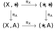
Let (X,Y,L) be a minmax problem.
Then there is a canonical commutative diagram
Proof
- May 6, 2024
- Eigil Fjeldgren Rischel
Proof
- May 6, 2024
- Eigil Fjeldgren Rischel
Proposition Slater's Constraint Qualification [lcc-002L]
- May 18, 2024
- Eigil Fjeldgren Rischel
Proposition Slater's Constraint Qualification [lcc-002L]
- May 18, 2024
- Eigil Fjeldgren Rischel
Consider an optimization problem in standard form:
- Minimize f_0(x), x \in \mathbb {R}^k
- Subject to f_1(x), \dots , f_n(x) \leq 0
- And g_1(x), \dots , g_m(x) = 0
- With each f_i convex and each g_i affine
Note: This is usually stated for a function defined on an arbitrary convex subset of \mathbb {R}^k. In this case we must further ask that x_0 is in the relative interior of this domain.
Proof
- May 18, 2024
- Eigil Fjeldgren Rischel
Proof
- May 18, 2024
- Eigil Fjeldgren Rischel
(Proof adapted from )
For simplicity, we will assume l = 0, i.e we will not assume any of the f_i are affine, and f_u(x_0) \leq 0 for all i \geq 1. (This is the standard form of Slater's constraint qualification).
Let A, b be a matrix and vector so that (g_i(x)) = Ax - b. Then assume without loss of generality that A has full rank. (Suppose g_j is in the span of the other g_is. Then if the affine constraints are feasible at all, the equation corresponding to g_j must be a consequence of the others. Hence we can delete g_j without altering the primal optimal value, and given a dual optimal value for the problem with g_j deleted, just set \nu _j = 0.)
Let \mathcal {A} = \{(u,v,t) \mid x \in \mathbb {R}^k, u_i \geq f_i(x), v_i = g_i(x), t \geq f_0(x)\} Observe that the optimal value is p^* = \inf _{(0,0,t) \in \mathcal {A}} t. Let \mathcal {B} = \{(0,0,t) \mid s \leq p^*\}. It's not hard to see that these sets are disjoint and convex, and hence there exists a hyperplane separating them. In other words, there exists \tilde {\lambda },\tilde {\nu },\tilde {\mu },\alpha (not all 0) so that (u,v,t) \in \mathcal {A} \Rightarrow \langle \tilde {\lambda },u \rangle + \langle \tilde {\nu },v \rangle + \mu t \geq \alpha (u,v,t) \in \mathcal {B} \Rightarrow \langle \tilde {\lambda },u \rangle + \langle \tilde {\nu },v \rangle + \mu t \leq \alpha By the first inequality, we must have \tilde {\lambda } \geq 0 (or the right-hand side would be unbounded below on \mathcal {A}, which is impossible). Similarly we have \mu \geq 0. The latter of the two statements is equivalent to the statement that \mu t \leq \alpha when t \leq p^*, which simply means \mu p^* \leq \alpha . Combining this with the first statement, we get for all x, \sum _i \tilde {\lambda }_i f_i(x) + \sum _i \tilde {nu}_i g_i(x) + \mu f_0(x) \geq \alpha \geq \mu p^*.
First assume \mu \neq 0. Then we can divide out and get L(x, \tilde {\lambda }/\mu , \tilde {\nu }/\mu ) \geq p^*, which proves that (\tilde {\lambda }/\mu , \tilde {\nu }/\mu ) is a dual optimal value and that strong duality holds.
If \mu =0, we have for all x \sum _i \tilde {\lambda }_i f_i(x) + \sum _i \tilde {nu}_i g_i(x) \geq 0
Inserting x_0, we find \sum _i \tilde {\lambda }_i f_i(x_0) \geq 0, and since f_i(x_0) = 0, we must have \tilde {\lambda } = 0. This then implies \sum _i \tilde {\nu }_i g_i(x) \geq 0 = \langle \tilde {nu},Ax - b \rangle for all x. But since this is an affine function, this can only be true if it's constantly zero. Since \tilde {\nu } is nonzero and A has full rank, this is impossible.
Theorem Minimax theorem [lcc-001E]
- April 22, 2024
- Eigil Fjeldgren Rischel
Theorem Minimax theorem [lcc-001E]
- April 22, 2024
- Eigil Fjeldgren Rischel
Let (L,X,A) \in \mathsf {Minmax}. If X,A are both convex, compact subspaces of finite-dimensional vector spaces, and L is continuous, then strong duality holds for L, and moreover an equilibrium I \to L \otimes L^* exists.
This theorem can be derived from the Kakutani fixpoint theorem in a very similar way to the usual proof of Nash's theorem about general, non-zerosum games - although note that it is not a special case, since X and A may not be simplices, and the payoff function here is merely convex, not necessarily affine as it is for a game-theoretic game.
However, we will give a different proof, which uses the structure of \mathsf {Minmax} in a more direct way. Essentially, we will use compactness to reduce to the case of simplexes, then use an inductive argument to reduce to the case where X = A = \Delta ^1 = [0,1], which can be shown by a direct topological argument. The inductive step is a fiber sequence argument, where we use the characterization of strong duality in terms of the Beck-Chevalley property, Proposition [lcc-0029].
Definition Solvable pair [lcc-002T]
- May 21, 2024
- Eigil Fjeldgren Rischel
Definition Solvable pair [lcc-002T]
- May 21, 2024
- Eigil Fjeldgren Rischel
Let X,A be topological convex spaces. We say the pair (X,A) is a solvable pair if, for any continuous minmax problem L: X \times A \to \mathbb {R}, strong duality holds.
Proposition [lcc-002V]
- May 21, 2024
- Eigil Fjeldgren Rischel
Proposition [lcc-002V]
- May 21, 2024
- Eigil Fjeldgren Rischel
The pair ([0,1],[0,1]) (in other words, (\Delta ^1,\Delta ^1)) is solvable.
Proof
- May 21, 2024
- Eigil Fjeldgren Rischel
Proof
- May 21, 2024
- Eigil Fjeldgren Rischel
Let L: [0,1] \times [0,1] \to \mathbb {R} be a continuous minmax problem. Suppose strong duality does not hold. Then by adding a constant to L, we can arrange that \sup _\theta \inf _s L(s,\theta ) < 0 < \inf _s \sup _\theta L(s,\theta ).
Consider the set P = \{(s,\theta ) \mid L(s,\theta ) > 0\}. Since we must have \sup _\theta L(s,\theta ) > 0 for each s, the first projection P \to [0,1] must be surjective. Since each fiber is convex, and hence connected, and the projection [0,1] \times [0,1] \to [0,1] is open, P is connected. As an open connected subset of a convex space, it is path connected. Hence there exists some path \gamma (t) \in P where \gamma (0) = (0,\theta _0) and \gamma (1) = (1,\theta _1). In other words (picturing the square with the first coordinate horizontal), there exists a path from the left to the right side of the cube so that L(\gamma (t)) > 0 everywhere on the path. Dually, there also exists a path from top to bottom so that L is strictly negative everywhere on that path. But they must intersect somewhere, and this is a contradiction. Hence L must have a state or a costate, finishing the proof.
Proposition [lcc-002W]
- May 21, 2024
- Eigil Fjeldgren Rischel
Proposition [lcc-002W]
- May 21, 2024
- Eigil Fjeldgren Rischel
Let E \to B be a continuous, affine map between topological convex spaces. Let A be another topological convex space, and suppose
- (B,A) is solvable.
- For every b \in B, (E_b,A) is solvable, where E_b \subseteq E is the fiber.
Proof
- May 21, 2024
- Eigil Fjeldgren Rischel
Proof
- May 21, 2024
- Eigil Fjeldgren Rischel
Recall that (E,A) being solvable means the following square has the Beck-Chevalley condition for continuous L:
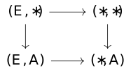
Now we can factor this as follows:
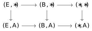
Note that the right-hand square here has the Beck-Chevalley condition by assumption. So it suffices to show the left-hand square does. For a given L, this means showing that these two functions on B are the same b \mapsto \inf _{e \mapsto b} \sup _a L(e,a) b \mapsto \sup _a \inf _{e \mapsto b} L(e,a) But this equation, for some given b, is exactly strong duality in the restriction of L to (E_b,A), which must hold because this is a solvable pair by assumption.
Corollary
- May 21, 2024
- Eigil Fjeldgren Rischel
Corollary
- May 21, 2024
- Eigil Fjeldgren Rischel
If (X,[0,1]) is solvable, so is (X,\Delta ^n) for each n, because the map \Delta ^n \to [0,1] which picks out the first coordinate has fibers isomorphic to \Delta ^{n-1}, so we can proceed by induction (the case n=0 being trivial.)
Lemma [lcc-002X]
- May 21, 2024
- Eigil Fjeldgren Rischel
Lemma [lcc-002X]
- May 21, 2024
- Eigil Fjeldgren Rischel
Let X be a compact topological convex space. Suppose (X,\Delta ^n) is solvable for all n. Then (X,A) is solvable for all topological convex spaces A.
Proof
- May 21, 2024
- Eigil Fjeldgren Rischel
Proof
- May 21, 2024
- Eigil Fjeldgren Rischel
Corollary [lcc-002Y]
- May 21, 2024
- Eigil Fjeldgren Rischel
Corollary [lcc-002Y]
- May 21, 2024
- Eigil Fjeldgren Rischel
If X is compact, (X,A) is solvable for any A.
Proof
- May 21, 2024
- Eigil Fjeldgren Rischel
Proof
- May 21, 2024
- Eigil Fjeldgren Rischel
- April 30, 2024
- Eigil Fjeldgren Rischel
- April 30, 2024
- Eigil Fjeldgren Rischel
By Corollary [lcc-002Y], the pair (X,A) is solvable, and strong duality holds. Since X,A are both compact, there must exist x^*,a^* attaining the infimum \inf _x \sup _a L(x,a) and the supremum \sup _a \inf _x L(x,a). These form an equilibrium.
It is interesting to note the use of compactness here. Recall that topological compactness is closely connected with the property, also called compactness, of \operatorname {\mathrm {Hom}}(X,-) preserving filtered colimits (this property, instantiated in \mathsf {Top}, is not actually the same thing as topological compactness). Our use of compactness here, to derive from the existence of a state in the "finitary" subproblems (L,X,\Delta ^n) the existence of a state in the entire problem, does not have this form (nor is it even the case that A is the colimit of its subsimplices), but it's possible that the proof could be rewritten to make this step more categorical.
The idea of proceeding by induction on n was inspired by Reference [weinstein-elementary-minimax-2022], although our proof is rather different - they are only looking at affine games, and hence their induction step is completely different (and they have no need for the complicated n=1 base case that we do), and since we are not merely interested in games on simplices, we need an additional compactness argument.
We can use the minimax theorem to derive other statements of interest about convex optimization
Theorem The separating hyperplane theorem (compact case) [lcc-002Z]
- May 22, 2024
- Eigil Fjeldgren Rischel
Theorem The separating hyperplane theorem (compact case) [lcc-002Z]
- May 22, 2024
- Eigil Fjeldgren Rischel
Let X,Y \subset \mathbb {R}^k be disjoint, compact, convex subspaces. Then there exists v \in \mathbb {R}^k and \alpha \in \mathbb {R} so that \langle v,x \rangle + \alpha < 0 < \langle v,y \rangle + \alpha whenever x \in X, y \in Y.
Proof
- May 22, 2024
- Eigil Fjeldgren Rischel
Proof
- May 22, 2024
- Eigil Fjeldgren Rischel
Consider the minmax problem
(L,X \times Y, A = \overline {B(0,1)} \subseteq \mathbb {R}^k), L(x,y,v) = \langle v,y-x \rangle .Since the closed unit ball is compact, by the minimax theorem there exists an equilibrium x^*,y^*,v^*, which then satisfies \langle v,y^*-x^* \rangle \leq \langle v^*,y^*-x^* \rangle \leq \langle v^*,y-x \rangle
By disjointness, y^*-x^* must be nonzero, so with a suitable choice of v we can clearly make the left-hand item strictly positive. Hence \langle v^*,y^*-x^* \rangle =: \delta > 0. Now there must exist some \alpha \in \mathbb {R} so that \langle v^*,y^* \rangle + \alpha = -\langle v^*,x^* \rangle - \alpha = \delta /2 > 0.
By the equilibrium property, we see that y^* must minimize \langle v^*,y \rangle on Y, and analogously x^* must maximize \langle v^*,x \rangle on X. Hence for all x,y, we have \langle v^*,x \rangle + \alpha \leq -\delta /2 < 0 < \delta /2 \leq \langle v^*,y \rangle + \alpha , which concludes the proof.
Theorem The separating hyperplane theorem (general case) [lcc-0030]
- May 22, 2024
- Eigil Fjeldgren Rischel
Theorem The separating hyperplane theorem (general case) [lcc-0030]
- May 22, 2024
- Eigil Fjeldgren Rischel
Let X,Y \subseteq \mathbb {R}^k be disjoint convex subsets. Then there exists v,\alpha so that \langle v,x \rangle + \alpha \leq 0 \leq \langle v,y \rangle + \alpha for all x \in X, y \in Y.
Proof
- May 22, 2024
- Eigil Fjeldgren Rischel
Proof
- May 22, 2024
- Eigil Fjeldgren Rischel
Let K_i, L_i, i=1, \dots be two sequences of sets with the following properties:
- For each i, K_i,L_i are disjoint.
- For each i, K_i \subseteq K_{i+1}
- Each of the K_i,L_i are compact and convex
- \cup _i K_i = X, \cup _i L_i = Y
Now apply Theorem [lcc-002Z] to obtain a sequence of v_i \in \overline {B(0,1)} so that \langle v_i,- \rangle is negative on K_i and positive on L_i. By compactness of the unit ball, this sequence has a point of density v^*. Now for every pair x \in X, y \in Y, we can find some i so that \langle v_i,x \rangle is within an arbitrary \epsilon of \langle v^*,x \rangle and the same is true for y, and so that x \in K_i, y \in L_i. But then \langle v^*,y-x \rangle is within 2\epsilon of \langle v_i,y-x \rangle , which is positive, so that \langle v^*,y-x \rangle \geq 0.
Now for each i, \langle v^*,- \rangle has a maximizer x_i^* on K_i and a minimizer y_i^* on L_i. Hence, by an argument analogous to the proof of Theorem [lcc-002Z], there is a nonempty closed interval [a_i,b_i] so that, if \alpha \in [a_i,b_i], we have \langle v^*,- \rangle + \alpha \leq 0 on K_i and \geq 0 on L_i. But since the sets K_i, L_i are increasing this sequence of intervals must be decreasing, and hence the intersection must be nonempty - and then any \alpha in this intersection will make \langle v^*,- \rangle + \alpha nonpositive on X, nonnegative on Y, as desired.
The Legendre Transform
- April 30, 2024
-
Eigil Fjeldgren Rischel
The Legendre Transform
- April 30, 2024
- Eigil Fjeldgren Rischel
Definition Convex conjugate [lcc-001P]
- April 25, 2024
-
Eigil Fjeldgren Rischel
Definition Convex conjugate [lcc-001P]
- April 25, 2024
- Eigil Fjeldgren Rischel
Let V be a (real) vector space, and f: V \to \mathbb {R} be a function (not necessarily linear). Then the convex conjugate f^*: V^* \to \mathbb {R} is defined by f^*(\alpha ) = \sup _x \alpha (x) - f(x)
The convex conjugate is also called the Legendre transform or the Fenchel-Legendre transform. It is intimately related to convex duality. We will prove the following fundamental property of the convex conjugate using the categorical language of minmax problems, and along the way we will see the role that convex duality plays. Note that our invocation of the term "strong duality" here is somewhat more complicated than strictly necessary - normally one would merely invoke the separating hyperplane theorem directly.
Proposition [lcc-001Q]
- April 25, 2024
-
Eigil Fjeldgren Rischel
Proposition [lcc-001Q]
- April 25, 2024
- Eigil Fjeldgren Rischel
Let f: V \to \mathbb {R} be convex, so that (V,*,f) is a minmax problem. Then we can form the modified minmax problem L = (V,V^*,(x,\alpha ) \mapsto f(x) - \alpha (x)) - note that, up to a sign change in the domain, this amounts to adding the constraint x = 0.
Then (L^*)^+ = -L^- = f^*
Note that the two uses of the asterisk in this equation conflict. We have both the reversed optimization problem L^* given by flipping the variables, and the convex conjugate function f^*. It may be good to alter this notation to resolve the conflict.
Proposition [lcc-001T]
- April 25, 2024
-
Eigil Fjeldgren Rischel
Proposition [lcc-001T]
- April 25, 2024
- Eigil Fjeldgren Rischel
Given a minmax problem L = (X,Y,L) where X is a finite-dimensional real vector space, let L|_{0} = (X, Y \oplus X^*, L \oplus - \langle -,- \rangle ) Note that (L|_0)^+(x) = \infty when x = 0 and L^+(0) otherwise. Thus this amounts to adding a constraint that x = 0. Analogously, define L|^0 = (L^*|_0)^* = (X \oplus Y^*, Y, L \oplus \langle -, - \rangle )
Then the Legendre transform f^* = ((f|_0)^*)^+ (viewing both f and f^* as minmax problems using the inclusion \mathsf {Conv} \to \mathsf {Minmax})
Proposition [lcc-001U]
- April 25, 2024
-
Eigil Fjeldgren Rischel
Proposition [lcc-001U]
- April 25, 2024
- Eigil Fjeldgren Rischel
Let f: X \to \mathbb {R} be a continuous convex function defined on a vector space. Then there is strong duality in the minmax problem f|_0
Proof
- April 25, 2024
- Eigil Fjeldgren Rischel
Proof
- April 25, 2024
- Eigil Fjeldgren Rischel
Observe that \{x,t \mid f(x) \leq t\} \subseteq X \oplus \mathbb {R} is a closed convex set. Hence there is a hyperplane through (0,f(0)) so that the entire set is in one half-space. This means a nontrivial affine equation A(x,t) \geq b which is satisfied whenever t \geq f(x), and where A(0,f(0)) = b.
Clearly A(x,t) = \alpha _0(x) - at for some \alpha _0 \in X^*, a \in \mathbb {R}. If a = 0 we have \alpha _0(x) \leq b for all x, which impossible. So by normalizing let's set a = 1. This means \alpha _0 (x) + f(x) \geq b = f(0).
Recall that the minmax problem f|_0 is given by (X,X^*,L(x,\alpha ) \mapsto f(x) - \alpha (x)). Strong duality means \inf _x\sup _\alpha L(x,\alpha ) = \sup _\alpha \inf _x L(x,\alpha ). We always have the inequality \geq , so it suffices to identify an \alpha ^* so that \inf _x \sup _\alpha L(x,\alpha ) \leq \inf _x L(x,\alpha ^*)
Clearly, for our L, we have \inf _x\sup _\alpha L(x,\alpha ) = f(0), since the supremum is \infty unless x = 0. On the other hand, taking \alpha ^* = -\alpha _0, we have f(0) \leq f(x) - \alpha ^*(x) for all x by construction, finishing the proof.
Lemma [lcc-003C]
- June 4, 2024
-
Eigil Fjeldgren Rischel
Lemma [lcc-003C]
- June 4, 2024
- Eigil Fjeldgren Rischel
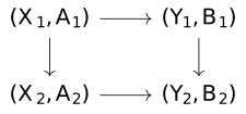
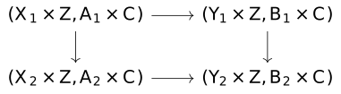
Given a commutative square:
Proposition [lcc-001V]
- April 25, 2024
-
Eigil Fjeldgren Rischel
Proposition [lcc-001V]
- April 25, 2024
- Eigil Fjeldgren Rischel
Let f be a convex function. Then f = (f^*)^* (where f^* denotes the Legendre transform), under the identification (X^*)^* = X of a finite-dimensional vector space with its double dual.
Proof
- April 25, 2024
- Eigil Fjeldgren Rischel
Proof
- April 25, 2024
- Eigil Fjeldgren Rischel
Recall that f^* = ((f|_0)^*)^+, as a minmax problem. Then the claim is that (((((f|_0)^*)^+)|_0)^*)^+ = f. Using first the rewrite ((-)^*)^+ = ((-)^-)^*, and the notation ((-)^*|_0)^* = -|^0, we can rewrite that as ((f|_0)^-|^0)^+
Now observe that, restricted to the subcategory \mathsf {Minmax}_l given by minmax problems (X,Y,L) where X,Y are real vector spaces, and those homomorphisms given by linear (rather than merely affine) maps, (-)|_0 and -|^0 form endofunctors, and (-)|_0 \dashv (-)|^0.
Since (-)^- is left adjoint to the inclusion, we have (-)|_0^- \dashv -|^0. Hence there is a canonical map, the unit of the adjunction, L \to (L|_0)^-|^0 for any L. If L = (X,*,f) is an element of \mathsf {Conv}, then by the universal property, this map factors over ((f|_0)^-|^0)^+. This gives us the inequality f \geq (f^*)^*.
(Note that this inequality actually holds even if f is not convex, and indeed we haven't really used convexity yet).
Observe that, using the natural identification (X^*)^* = X, we have (f|_0)|^0 = (X \oplus X, X^*, (x,x';\alpha ) \mapsto f(x) - \alpha (x) + \alpha (x')). Clearly \inf _x \sup _\alpha f(x) - \alpha (x) + \alpha (x') = f(x'), since the supremum is infinite unless x = x'. But observe that (f^*)^*(x') = \sup _\alpha \inf _x f(x) - \alpha (x) + \alpha (x')
Our claim now is that we may exchange these extremizers by strong duality. This amounts to the claim that the local Beck-Chevalley property holds for this square at (f|_0)|^0:
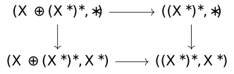
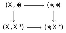
But by Proposition [lcc-001U], strong duality holds in every square of the form
Misc stuff (sorting)
- April 30, 2024
-
Eigil Fjeldgren Rischel
Misc stuff (sorting)
- April 30, 2024
- Eigil Fjeldgren Rischel
Composition of minmax problems [lcc-001Y]
- April 26, 2024
-
Eigil Fjeldgren Rischel
Composition of minmax problems [lcc-001Y]
- April 26, 2024
- Eigil Fjeldgren Rischel
Let Y be a real vector space, and let (X,Y,L), (Y^*,Z,L) be minmax problems. Then we can try to define a composite minmax problem L\circ _Y L'(x,z) = \sup _y \inf _{y'} L(x,y) + L(y',z) - y'(y)
For this composition to be associative relies on a strong duality property. We probably shouldn't want to treat this as well-defined unless it holds.
Note that by the convex duality stuff, the minmax problem Y^*,Y,\operatorname {ev} acts as an identity for this composition.
This may fit together into a double category type structure for minmax problems (maybe restricted to linear maps between the spaces).
Minmax problems are not star-autonomous [lcc-001M]
- April 23, 2024
-
Eigil Fjeldgren Rischel
Minmax problems are not star-autonomous [lcc-001M]
- April 23, 2024
- Eigil Fjeldgren Rischel
Since the category of minmax problems is very similar to a Chu construction, we might hope that we could define a similar star-autonomous structure on minmax problems. Unfortunately, this does not work. We do have the duality, Dual minmax problem, but it doesn't extend to a star-autonomous structure.
Morally speaking, the tensor product of (X,Y,L), (X',Y',L') would be given by X \otimes X' in the forwards direction, and pairs of affine functions f: X \to Y', g: X' \to Y satisfying L(x,g(x')) = L'(x',f(x)) in the backwards direction, with either of these expressions giving the pairing. Since the first formula implies the pairing is convex in x (as it must be), but the latter implies it's concave in x, g must take values only those y so that L(-,y) is affine, and similarly for f. This can easily be an empty set, but in a star-autonomous category we always have a canonical costate L \otimes L^* \to I, which would be impossible in that case.
Proposition [lcc-001K]
- April 23, 2024
-
Eigil Fjeldgren Rischel
Proposition [lcc-001K]
- April 23, 2024
- Eigil Fjeldgren Rischel
The category of minmax problems has products, given by (X,Y,L) \times (X',Y',L') = (X \times X', Y \oplus Y', (L \times L')), (L \times L')(x,x'; \alpha y + \beta y') = \alpha L(x,y) + \beta L'(x',y')
(L \times L')^+(x,x') = \max (L^+(x),L'^+(x'))
Here Y \oplus Y' denotes the coproduct of convex spaces, and \alpha y + \beta y' is a generic element (note that \alpha ,\beta \in [0,1], \alpha + \beta = 1)
By duality (with (-)^*), it also has coproducts given by (X,Y,L) \oplus (X',Y',L') = (X \oplus X', Y \times Y', L(\alpha x + \beta x';y,y') = \alpha L(x,y) + \beta L'(x',y')).
 @article
{rischel-cvxdual-2025, title={Convex Duality Made Difficult}, volume={??}, journal={EPTCS}, author={Rischel, Eigil Fjeldgren}, pages={1–14}, date={2025} }
Reference Representable Markov categories and comparison of statistical experiments in categorical probability [fritz-gonda-perrone-rischel-rep]
- June 15, 2023
-
Tobias Fritz, Tomas Gonda, Paolo Perrone, Eigil Fjeldgren Rischel
-
10.1016/j.tcs.2023.113896
Reference Representable Markov categories and comparison of statistical experiments in categorical probability [fritz-gonda-perrone-rischel-rep]
- June 15, 2023
- Tobias Fritz, Tomas Gonda, Paolo Perrone, Eigil Fjeldgren Rischel
- 10.1016/j.tcs.2023.113896
Abstract
- June 15, 2023
-
Tobias Fritz, Tomas Gonda, Paolo Perrone, Eigil Fjeldgren Rischel
Abstract
- June 15, 2023
- Tobias Fritz, Tomas Gonda, Paolo Perrone, Eigil Fjeldgren Rischel
Markov categories are a recent categorical approach to the mathematical foundations of probability and statistics. Here, this approach is advanced by stating and proving equivalent conditions for second-order stochastic dominance, a widely used way of comparing probability distributions by their spread. Furthermore, we lay the foundation for the theory of comparing statistical experiments within Markov categories by stating and proving the classical Blackwell-Sherman-Stein Theorem. Our version not only offers new insight into the proof, but its abstract nature also makes the result more general, automatically specializing to the standard Blackwell-Sherman-Stein Theorem in measure-theoretic probability as well as a Bayesian version that involves prior-dependent garbling. Along the way, we define and characterize representable Markov categories, within which one can talk about Markov kernels to or from spaces of distributions. We do so by exploring the relation between Markov categories and Kleisli categories of probability monads.
 @article
{fritz-gonda-perrone-rischel-rep, title={Representable Markov categories and comparison of statistical experiments in categorical probability}, volume={961}, ISSN={0304-3975}, DOI={10.1016/j.tcs.2023.113896}, journal={Theoretical Computer Science}, author={Fritz, Tobias and Gonda, Tomas and Perrone, Paolo and Fjeldgren Rischel, Eigil}, year={2023}, month={Jun}, pages={113896} }
Reference Towards Foundations of Categorical Cybernetics [towards-cybercat]
- November 3, 2022
-
Matteo Capucci, Bruno Gavranović, Jules Hedges, Eigil Fjeldgren Rischel
-
10.4204/EPTCS.372.17
Reference Towards Foundations of Categorical Cybernetics [towards-cybercat]
- November 3, 2022
- Matteo Capucci, Bruno Gavranović, Jules Hedges, Eigil Fjeldgren Rischel
- 10.4204/EPTCS.372.17
Abstract
- November 3, 2022
-
Matteo Capucci, Bruno Gavranović, Jules Hedges, Eigil Fjeldgren Rischel
Abstract
- November 3, 2022
- Matteo Capucci, Bruno Gavranović, Jules Hedges, Eigil Fjeldgren Rischel
We propose a categorical framework for processes which interact bidirectionally with both an environment and a “controller”. Examples include open learners, in which the controller is an optimiser such as gradient descent, and an approach to compositional game theory closely related to open games, in which the controller is a composite of game-theoretic agents. We believe that “cybernetic” is an appropriate name for the processes that can be described in this framework.
@article
{towards-cybercat, title={Towards Foundations of Categorical Cybernetics}, volume={372}, ISSN={2075-2180}, DOI={10.4204/EPTCS.372.17}, url={https://arxiv.org/abs/2105.06332}, journal={Electronic Proceedings in Theoretical Computer Science}, author={Capucci, Matteo and Gavranović, Bruno and Hedges, Jules and Rischel, Eigil Fjeldgren}, year={2022}, month={Nov}, pages={235–248} }
Reference Fibre optics [fibre-optics-2021]
- December 21, 2021
-
Dylan Braithwaite, Matteo Capucci, Bruno Gavranović, Jules Hedges, Eigil Fjeldgren Rischel
-
10.48550/arXiv.2112.11145
-
http://arxiv.org/abs/2112.11145
Reference Fibre optics [fibre-optics-2021]
- December 21, 2021
- Dylan Braithwaite, Matteo Capucci, Bruno Gavranović, Jules Hedges, Eigil Fjeldgren Rischel
- 10.48550/arXiv.2112.11145
- http://arxiv.org/abs/2112.11145
Abstract
- December 21, 2021
-
Dylan Braithwaite, Matteo Capucci, Bruno Gavranović, Jules Hedges, Eigil Fjeldgren Rischel
Abstract
- December 21, 2021
- Dylan Braithwaite, Matteo Capucci, Bruno Gavranović, Jules Hedges, Eigil Fjeldgren Rischel
Lenses, optics and dependent lenses (or equivalently morphisms of containers, or equivalently natural transformations of polynomial functors) are all widely used in applied category theory as models of bidirectional processes. From the definition of lenses over a finite product category, optics weaken the required structure to actions of monoidal categories, and dependent lenses make use of the additional property of finite completeness (or, in case of polynomials, even local cartesian closure). This has caused a split in the applied category theory literature between those using optics and those using dependent lenses. The goal of this paper is to unify optics with dependent lenses, by finding a definition of fibre optics admitting both as special cases.
 @article
{fibre-optics-2021, title={Fibre optics}, url={http://arxiv.org/abs/2112.11145}, DOI={10.48550/arXiv.2112.11145}, number={arXiv:2112.11145}, publisher={arXiv}, author={Braithwaite, Dylan and Capucci, Matteo and Gavranović, Bruno and Hedges, Jules and Rischel, Eigil Fjeldgren}, year={2021}, month={Dec} }
Reference Compositional abstraction error and a category of causal models [rischel_compositional_2021]
- August 5, 2021
-
Eigil Fjeldgren Rischel, Sebastian Weichwald
-
10.48550/arXiv.2103.15758
Reference Compositional abstraction error and a category of causal models [rischel_compositional_2021]
- August 5, 2021
- Eigil Fjeldgren Rischel, Sebastian Weichwald
- 10.48550/arXiv.2103.15758
Abstract
- August 5, 2021
-
Eigil Fjeldgren Rischel, Sebastian Weichwald
Abstract
- August 5, 2021
- Eigil Fjeldgren Rischel, Sebastian Weichwald
Interventional causal models describe several joint distributions over some variables used to describe a system, one for each intervention setting. They provide a formal recipe for how to move between the different joint distributions and make predictions about the variables upon intervening on the system. Yet, it is difficult to formalise how we may change the underlying variables used to describe the system, say moving from fine-grained to coarse-grained variables. Here, we argue that compositionality is a desideratum for such model transformations and the associated errors: When abstracting a reference model M iteratively, first obtaining M' and then further simplifying that to obtain M'', we expect the composite transformation from M to M'' to exist and its error to be bounded by the errors incurred by each individual transformation step. Category theory, the study of mathematical objects via compositional transformations between them, offers a natural language to develop our framework for model transformations and abstractions. We introduce a category of finite interventional causal models and, leveraging theory of enriched categories, prove the desired compositionality properties for our framework.
@misc{rischel_compositional_2021,
 author = {Rischel, Eigil F. and Weichwald, Sebastian},
 date = {2021-08-05},
 doi = {10.48550/arXiv.2103.15758},
 eprint = {2103.15758 [cs, math, stat]},
 eprinttype = {arxiv},
 keywords = {Computer Science - Artificial Intelligence, Computer Science - Logic in Computer Science, Computer Science - Machine Learning, Mathematics - Category Theory, Statistics - Machine Learning},
 number = {{arXiv}:2103.15758},
 publisher = {{arXiv}},
 title = {Compositional Abstraction Error and a Category of Causal Models},
 url = {http://arxiv.org/abs/2103.15758},
 urldate = {2024-05-25}
}
Reference Infinite products and zero-one laws in categorical probability [rischel-fritz-infinite-products]
- August 11, 2020
-
Tobias Fritz, Eigil Fjeldgren Rischel
-
10.32408/compositionality-2-3
Reference Infinite products and zero-one laws in categorical probability [rischel-fritz-infinite-products]
- August 11, 2020
- Tobias Fritz, Eigil Fjeldgren Rischel
- 10.32408/compositionality-2-3
Abstract
- August 11, 2020
-
Tobias Fritz, Eigil Fjeldgren Rischel
Abstract
- August 11, 2020
- Tobias Fritz, Eigil Fjeldgren Rischel
We state and prove the zero-one laws of Kolmogorov and Hewitt-Savage within the setting of Markov categories, a category-theoretic approach to the foundations of probability and statistics. This gives general versions of these results which can be instantiated not only in measure-theoretic probability, where they specialize to the standard ones in the setting of standard Borel spaces, but also in other contexts. For example, applying the Kolmogorov law to the Kleisli category of the hyperspace monad on topological spaces gives criteria for when maps out of an infinite product of topological spaces into a Hausdorff space are constant.
 @article
{rischel-fritz-infinite-products, title={Infinite products and zero-one laws in categorical probability}, volume={2}, ISSN={2631-4444}, DOI={10.32408/compositionality-2-3}, journal={Compositionality}, author={Fritz, Tobias and Rischel, Eigil Fjeldgren}, year={2020}, month={Aug}, pages={3},language={en} }
Blog [efr-AE01]
- October 15, 2025
-
Eigil Fjeldgren Rischel
Blog [efr-AE01]
- October 15, 2025
- Eigil Fjeldgren Rischel
A simple categorical proof of (a) Martingale Convergence Theorem [efr-5NUC]
- October 13, 2025
-
Eigil Fjeldgren Rischel
A simple categorical proof of (a) Martingale Convergence Theorem [efr-5NUC]
- October 13, 2025
- Eigil Fjeldgren Rischel
Theorem
- October 13, 2025
-
Eigil Fjeldgren Rischel
Theorem
- October 13, 2025
- Eigil Fjeldgren Rischel
Let \Omega _1 \leftarrow \Omega _2 \leftarrow \dots be a sequence of probability spaces, for example \Omega _i = (\Omega , \mathcal {F}_i, P) for some filtration of sigma-algebras. A martingale on this object is a sequence of random variables defined on \Omega _i so that E[X_{i+1} \mid \Omega _i] = X_i. Let \Omega _\infty denote the limit of this diagram in probability spaces. Then every martingale of L^2-random variables defines a sequence of random variables on \Omega _\infty . This sequence converges in L^2, say to X_\infty , and X_n = E[X_\infty \mid \Omega _n]
Proof
- October 13, 2025
- Eigil Fjeldgren Rischel
Proof
- October 13, 2025
- Eigil Fjeldgren Rischel
Note that L^2(-) defines a contravariant functor from probability spaces to Hilbert spaces and bounded maps. This functor carries the limit \Omega _\infty = \lim _i \Omega _i to a colimit. To see this, first note that it carries each map to an embedding (since every measure-preserving map is onto up to a set of measure zero), so it suffices to show that every L^2 measurable function f on the limit is a limit of functions f_i which factor over \Omega _i.
Let such an f be given. Fix K so that the L^2-norm of the part of f outside [-K,K] is small. Partition [-K,K] into intervals of width 1/i. Each of the sets f^{-1}([ k/i, k+1/i )) is measurable. Hence there is some N_i so that each of these intervals is approximated up to probability \epsilon / i by some \Omega _{N_i}-measurable set. Define f_i to be equal to k/i on these approximating sets and zero outside of that. Then f_i is within 2\epsilon of f in L^2.
Now since forming adjoints is a self-duality on Hilbert spaces, this immediately implies that L^2(\Omega _\infty ) is also the inverse limit of the adjoint diagram, where the map L^2(\Omega _{i+1}) \to L^2(\Omega _i) is given by conditional expectation. It is apparent that an element of this inverse limit is precisely a martingale. Hence every martingale is the conditional expectation of a unique L^2-function on \Omega _\infty . It's clear that if a martingale converges, it is the conditional expectation of its limit, so we only need to show that given f \in L^2(\Omega _\infty ), E[f \mid \Omega _i] \to f.
Since the union of the inclusions L^2(\Omega _i) \hookrightarrow L^2(\Omega _\infty ) is dense, this is straightforward.
This concept is essentially what is called a bilimit in domain theory and studied for embedding-projection pairs.
Against calibration [againstcalibration]
- September 28, 2023
-
Eigil Fjeldgren Rischel
Against calibration [againstcalibration]
- September 28, 2023
- Eigil Fjeldgren Rischel
Forecasting is predicting whether something will happen, like who will be the next US president or whether a natural disaster will happen or what the economy is going to be like in a year. It's notoriously difficult to think about. Typically who study this sort of thing think you should make quantifiable predictions with specific probabilities assigned to them, make them public, and then let people rate your performance later to figure out who's good at forecasting. I'm not gonna explain all this in too much detail. See eg the discussion at the start of this astralcodexten post.
One way to rate forecasts is "Brier score".[^2] If you assign something probability p, and it happens, your Brier score is (1-p)^2. If it doesn't happen, your Brier score is p^2 (since you essentially said it wouldn't happen with probability 1-p). Lower is better - the lowest possible Brier score is 0, the highest is 1. If you make many predictions, your Brier score is the average Brier score across the whole set of questions.
Another way to rate forecasters is "calibration". Calibration looks at the fraction of your "X% likely" predictions that occurred, and asks how close that fraction is to X% (for each X). Then you can plot it in graphs like this (source: Manifold on twitter):
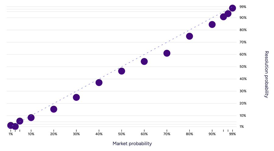
On average, clearly, 10% of your 10% predictions should come true if you're assigning probabilities sensibly, so it seems good to have good calibration. Brier scoring agrees with this, in the following sense: suppose in fact 14% of your 10% predictions come true. Then you would have obtained a higher Brier score by replacing all your 10% predictions with 14%[^1].
[^1]: This is essentially what people mean when they say Brier scoring is a "proper scoring rule".
There are a few reason people focus on calibration
- Perhaps most importantly, it's *comparable across question sets*. That is, if I make a bunch of predictions, and you make a *different set* of predictions, we can sensibly compare our calibration plots and see who did better. In contrast, predicting more difficult question sets will result in a lower Brier score even if you're doing as well as possible (in the limit, predicting coinflips, if you assign the correct 50-50 probability you'll get an average Brier score of 0.25, whereas if you predict events that happen 10% of the time and assign that probability correctly you'll get a Brier score of 0.09).
- There's some evidence that calibration is *trainable* and *generalizes.* That is, if you practice, you can improve your calibration, and if your calibration is good on one type of questions (say, about politics), it'll tend to be good on other questions (about technological advances, say) as well.
These obviously make calibration a pretty useful concept, and I don't want to disparage that. It's good to practice your calibration if you want to make precise predictions, and it's good to publish your calibration graph if you want people to take your forecast seriously.
Calibration is a very weak statement about the quality of your forecasts
- September 28, 2023
-
Eigil Fjeldgren Rischel
Calibration is a very weak statement about the quality of your forecasts
- September 28, 2023
- Eigil Fjeldgren Rischel
Manifold (to their credit!) publishes their calibration plots. These are generally pretty good. Some people seem take this as strong evidence that Manifold makes good predictions.
We can try to think about perfect calibration in market terms. If some method could improve on Manifold's predictions, then that method could be turned into a profitable trading strategy. So we can think about statements that Manifold makes "good" predictions in terms of the classes of strategy they rule out. In the extreme case, if the market was perfectly efficient, no strategy could make a profit - meaning there's no way to improve the predictions.
Perfect calibration means that, (for example) of the markets currently trading at 10% YES, 10% will resolve YES. This means that no trading strategy of the type "whenever a market is valued at 10% YES, buy some of it" can make a profit in expectation. This is obviously an *incredibly weak* notion of market efficiency. We expect this to hold, but this doesn't mean the predictions are well-priced at all.
Good calibration doesn't mean you have a good Brier score
- September 28, 2023
-
Eigil Fjeldgren Rischel
Good calibration doesn't mean you have a good Brier score
- September 28, 2023
- Eigil Fjeldgren Rischel
Imagine two people forecasting the same set of 100 potential natural disasters. The first forecaster (call him A) assigns probability 1% to them all. The second forecaster (B) assigns probability 80% to two of them, and 2% to the rest. In the end, exactly one of the disasters happen, and it's one of the two that the second forecaster assigned 80% probability to.
A has perfect calibration. B, by contrast, has pretty bad calibration (his 80% "should" have been 50%, and his 2% should have been 0%).
But: - B has a better Brier score (A has (0.0099 + 0.99^2)/100, B has approximately (0.8^2 + 0.2^2 + 0.0004 \cdot 98) /100, and remember lower is better). - More to the point, B's forecast is *clearly more useful* - having some reasonable ideas *which* of the 100 potential disasters will happen is clearly more important than getting the overall rate right - We could make this point even more stark by letting B assign 90% probability to the disaster that ended up happening, and 1% probability to the ones that don't.
Good calibration doesn't mean other people should adopt your forecasts
- September 28, 2023
-
Eigil Fjeldgren Rischel
Good calibration doesn't mean other people should adopt your forecasts
- September 28, 2023
- Eigil Fjeldgren Rischel
People often say things like "X has good calibration, meaning when they say there's a 10% chance of something happening, it happens 10% of the time. So when they say there's a 10% chance of nuclear war (or whatever), we should take it seriously".
The first sentence is of course a correct explanation of calibration. But think of our disaster forecasters from before. A had perfect calibration, meaning when A says that disasters overall happen only one time in a hundred, he's right. But if he says that some *specific* disaster has a very low, 1%, probability of happening, we shouldn't necessarily take that forecast very seriously. Perhaps it's actually easy to know which 1% of disasters happen. A's ability to get the base rate right does say something about his forecasting, but the fact that he can't do better than the base rate doesn't prove that we can't, and should therefore adopt his forecast.
[^2]: Another is log scoring, where if you say X will happen with probability p and it happens, you score is -\log p instead of (1-p)^2. For our purposes the difference doesn't really matter (both have this property of being a "proper scoring rule", so if you have to assign the same probability to some set of questions, you optimize your score by assigning the fraction of them that comes out true).
Coproducts in the category of lenses [coprods-lens-blogpost]
- September 20, 2023
-
Eigil Fjeldgren Rischel
Coproducts in the category of lenses [coprods-lens-blogpost]
- September 20, 2023
- Eigil Fjeldgren Rischel
Introduction
- September 20, 2023
-
Eigil Fjeldgren Rischel
Introduction
- September 20, 2023
- Eigil Fjeldgren Rischel
The category of bimorphic lenses and its many generalizations has been widely studied and utilized in applied category theory. We will not give a review of the literature here, but see e.g. Riley's paper on "optics" (one of the many generalizations) Reference [riley-optics], which includes a decent overview.
Dispensing with a point of notation, we will denote objects of the category of lenses \binom {A}{X}, and morphisms \varphi : \binom {A}{X} \to \binom {B}{Y} as (\varphi ^+: X \to Y,\varphi ^- : X \times B \to A). Note that we write the *forwards* pass on the bottom of the tuple, breaking with the convention used by Riley and many others.
The category \mathsf {Lens}= \mathsf {Lens}(\mathsf {Set}) of lenses embeds into the category of polynomial functors \mathsf {Poly} and natural transformations as the full subcategory of functors of the form X \times (-)^A. Since \mathsf {Poly} admits all coproducts, and these are computed pointwise, one immediate consequence is that we have the coproducts \binom {A}{X} + \binom {A}{Y} = \binom {A}{X + Y} in \mathsf {Lens}. These seem to have been studied first by Hedges (Reference [hedges-morphisms-open-games]). (For a reference on \mathsf {Poly}, including this inclusion, see eg Spivak Reference [spivak-poly-abundant]. \mathsf {Poly} is another branch on the tree of generalizations of \mathsf {Lens}, studied extensively by Spivak and others).
Given the above, one might expect these to be all the coproducts of \mathsf {Lens} (up to isomorphism) - they are certainly the only ones preserved by this inclusion11 There is a quibble here, since \binom {A}{0} \cong \binom {B}{0} for any sets A,B, these being the initial objects of \mathsf {Lens}. This is of course the natural "nullary" version of the binary formula, but it also means that \binom {A}{0}+\binom {B}{X} = \binom {B}{X}, and that this coproduct is preserved by the inclusion into \mathsf {Poly}, even if A \not \cong B. . But this turns out not to be the case.
Let's begin with a worked example of the "exotic" coproducts. Note that I simply denote by n \in \mathbb {N} the set \{1, \dots n\} with n elements. In particular 0 is the empty set.
Example
- September 20, 2023
-
Eigil Fjeldgren Rischel
Example
- September 20, 2023
- Eigil Fjeldgren Rischel
In \mathsf {Lens}, \binom {0}{1} + \binom {1}{1} = \binom {0}{2}, with the coproduct inclusions having as their forwards pass the two distinct maps 1 \to 2, and the backwards passes in both cases being trivial.
To see this is a coproduct, consider the natural transformation
\mathsf {Lens}\left (\binom {0}{2},\binom {A}{X}\right ) \to \mathsf {Lens}\left (\binom {0}{1},\binom {A}{X}\right ) \times \mathsf {Lens}\left (\binom {1}{1},\binom {A}{X}\right )In the case where A is nonempty, this is simply the map 0 \to 0, because there are no maps 2 \times A \to 0, and also no maps 1 \times A \to 0. Clearly 0 \to 0 is a bijection. On the other hand if A is empty, all the backwards passes are trivial, so we're just left with the map \mathsf {Set}(2,A) \to \mathsf {Set}(1,A) \times \mathsf {Set}(1,A), which is clearly a bijection. Hence this is a natural isomorphism, so we have a coproduct.
To see why this is not preserved by the inclusion \mathsf {Lens}\hookrightarrow \mathsf {Poly}, consider the polynomial y \mapsto y + 1 (this is the actual coproduct of the polynomials corresponding to these lenses). The inclusion maps from y = 1 \times y^1 and 1 = 1 \times y^0 into this polynomial should induce a map from 2 = 2 \times y^0, but of course there's no way to map into the y (unless we map the entire thing into the 1 component, but this clearly won't pull back to the inclusion map of y when we compose with the map y \to 2). The problem is that, where in the lens/monomial case, to have any maps at all the backwards set must be 0, making the whole backwards pass trivial, in the polynomial case we can have the backwards set be empty only when it's forced to be.
The coproducts in \mathsf {Lens}
- September 20, 2023
-
Eigil Fjeldgren Rischel
The coproducts in \mathsf {Lens}
- September 20, 2023
- Eigil Fjeldgren Rischel
Having seen the above, we may begin to lose hope of understanding the coproducts in \mathsf {Lens} at all. Fortunately the situation is not completely chaotic - in some sense, the preceding example is the *only* problem - all the coproducts in \mathsf {Lens} are either of the form \binom {A}{\coprod _i X_i} (up to isomorphism), or they are of the same form as the example.
Theorem
- September 20, 2023
-
Eigil Fjeldgren Rischel
Theorem
- September 20, 2023
- Eigil Fjeldgren Rischel
In \mathsf {Lens}= \mathsf {Lens}(\mathsf {Set}), a tuple of lenses \{\binom {A_i}{X_i} \overset {\varphi _i}{\to } \binom {B}{Y}\} is a coproduct diagram if and only if the forwards passes \{X_i \to Y\} form a coproduct diagram in \mathsf {Set}, and one of these conditions hold:
- For all i, and for all x \in X_i, the function \varphi _i(x, -): B \to A_i is a bijection.
- For at least one i, A_i is empty and X_i is nonempty. (The existence of any lens \binom {A_i}{X_i} \to \binom {B}{Y} then implies that B must be empty as well)
The first class of coproducts are the "good" ones - these are preserved by the functor from lenses to polynomial functors, and seem to capture the correct notion of "branching" for bidirectional systems. The other class, the "exotic" coproducts, are more mysterious.
We will begin the proof of this theorem with some preliminaries about lenses in a general (Cartesian) distributive category. While we can't obtain the preceding theorem in this generality (for reasons that will become clear later), it may be useful to know what can be said here.
Let us fix a (Cartesian) distributive category \mathcal {C} - that is, \mathcal {C} has finite products and coproducts, and the universal map \coprod _i A \times X_i \to A \times (\coprod _i X_i) is always an isomorphism. I will denote the initial object by 0.
Proposition
- September 20, 2023
-
Eigil Fjeldgren Rischel
Proposition
- September 20, 2023
- Eigil Fjeldgren Rischel
The functor \mathsf {Lens}(\mathcal {C}) \to \mathcal {C} which carries \binom {A}{X} to X and a lens (\varphi ^+, \varphi ^-) to its foward pass \varphi ^+ admits a right adjoint, given by X \mapsto \binom {0}{X}.
Proof
- September 20, 2023
-
Eigil Fjeldgren Rischel
Proof
- September 20, 2023
- Eigil Fjeldgren Rischel
We simply have to verify \mathsf {Lens}(\mathcal {C})(\binom {A}{X},\binom {0}{Y}) = \mathcal {C}(X,Y). But this is trivial - the forwards pass of such a lens is clearly an element of the right-hand side, so it suffices to prove that there is always a unique choice of backwards pass. But the backwards pass is a map 0 \times X \to A, and by distributivity 0 \times X is initial. This concludes the proof.
Because left adjoints preserve (in particular) coproducts, we obtain the following:
Corollary
- September 20, 2023
-
Eigil Fjeldgren Rischel
Corollary
- September 20, 2023
- Eigil Fjeldgren Rischel
For a tuple \{\binom {A_i}{X_i} \overset {\varphi _i}{\to } \binom {B}{Y}\} to be a coproduct diagram, the forwards passes X_i \to Y must form a coproduct diagram in \mathcal {C}.
The following result, characterizing the "good" coproducts, was already essentially proven by Hedges in Reference [hedges-morphisms-open-games]22 Hedges states it only for \mathcal {C} = \mathsf {Set}, but his proof goes through unaltered for our case. He also only constructs a particular family of coproduct diagrams, but the ones considered here are just his composed with isomorphisms in \mathsf {Lens}, so there is really nothing serious going on , but I'll state it here and sketch a proof for completeness.
Proposition
- September 20, 2023
-
Eigil Fjeldgren Rischel
Proposition
- September 20, 2023
- Eigil Fjeldgren Rischel
Let X_i be a collection of objects of \mathcal {C}, and \coprod _i X_i a coproduct. Let also A \in \mathcal {C}. Then the family of lenses \binom {A}{X_i} \to \binom {A}{\coprod _i X_i} with forwards passes given by the coproduct inclusions, and backwards passes by the projection X_i \times A \to A, is a coproduct diagram.
Proof
- September 20, 2023
-
Eigil Fjeldgren Rischel
Proof
- September 20, 2023
- Eigil Fjeldgren Rischel
using the universal property of coproducts and the distributivity. This is clearly the set of tuples of lenses \binom {A}{X_i} \to \binom {B}{Y}, and moreover precomposition with the inclusion maps clearly picks out the elements of the tuple, verifying the universal property of the coproduct.
Proposition
- September 20, 2023
-
Eigil Fjeldgren Rischel
Proposition
- September 20, 2023
- Eigil Fjeldgren Rischel
Let a tuple \{\binom {A_i}{X_i} \overset {\varphi _i}{\to } \binom {B}{\coprod _i X_i}\} be given, such that each \varphi _i^+: X_i \to \coprod _j X_j is the coproduct inclusion.
Given some object C \in \mathcal {C}, each \varphi _i^-: X_i \times B \to A_i determines a map (\varphi _i^-)^*: \mathcal {C}(X_i \times C, B) \to \mathcal {C}(X_i \times C, A_i) , given by (\varphi _i^-)^*\psi (x,c) = \varphi _i^-(x,\psi (x,c)). The tuple (\varphi _i) is a coproduct diagram if and only if, for all C, one of these conditions hold (not necessarily the same one for each C):
1. Each (\varphi _i^-)^* is a bijection.
2. For some i, the set \mathcal {C}(X_i \times C, A_i) is empty.
Proof
- September 20, 2023
-
Eigil Fjeldgren Rischel
Proof
- September 20, 2023
- Eigil Fjeldgren Rischel
Note that each of the lenses \varphi _i factors as \binom {A_i}{X_i} \to \binom {B}{X_i} \to \binom {B}{\coprod X_i} = \coprod _i \binom {B}{X_i}, where the first map is (1_{X_i},\varphi _i^-), and the second map is the coproduct inclusion.
Hence the natural transformation
\alpha : \mathsf {Lens}(\mathcal {C})\left (\binom {B}{\coprod _i X_i},\binom {C}{Z}\right ) \to \prod _i \mathsf {Lens}(\mathcal {C})\left (\binom {A_i}{X_i},\binom {C}{Z}\right )factors as
\mathsf {Lens}(\mathcal {C})\left (\binom {B}{\coprod _i X_i},\binom {C}{Z}\right ) \cong \prod _i\mathsf {Lens}(\mathcal {C})\left (\binom {B}{X_i},\binom {C}{Z}\right ) \to \prod _i\mathsf {Lens}(\mathcal {C})\left (\binom {A_i}{X_i},\binom {C}{Z}\right )where the second map is the parallel product of the precomposition morphisms - \circ (1_{X_i},\varphi _i^-) for each i.
The tuple is a coproduct diagram if and only if this composite is a bijection, which is true if and only if this second map is a bijection.
A product of functions in \mathsf {Set} is a bijection if and only if each component map is a bijection, or one of the product sets in the target is empty (in which case the corresponding set in the domain must be empty as well for a map to exist, and so both products are empty).
We can rewrite the sets involved here as
\mathsf {Lens}(\mathcal {C})\left (\binom {B}{X_i},\binom {C}{Z}\right ) = \mathsf {Set}(X_i,Z) \times \mathsf {Set}(X_i \times C, B),and
\mathsf {Lens}(\mathcal {C})\left (\binom {A_i}{X_i},\binom {C}{Z}\right ) = \mathsf {Set}(X_i,Z) \times \mathsf {Set}(X_i \times C, A_i).This is simply the definition of \mathsf {Lens}
Under this expansion the map - \circ (1_{X_i},\varphi _i^-) carries a lens (\psi ^+, \psi ^-) to (\psi ^+, (\varphi _i^-)^*\psi ^-). So - \circ (1_{X_i},\varphi _i^-)i is a bijection if and only if we have \mathsf {Set}(X_i,Z) empty or (\varphi _i^-)^* a bijection (or both).
Now, clearly if condition 1. holds, we've just seen that each - \circ (1_{X_i},\varphi _i^-) becomes a bijection, and so our map \alpha is a bijection. If condition 2. holds, then \mathsf {Lens}(\mathcal {C})\left (\binom {A_i}{X_i},\binom {C}{Z}\right ) is empty, and so we again have a (trivial) bijection.
So if at least one of the conditions hold for each C, \alpha is always a bijection, and so we have a coproduct.
On the other hand, suppose there is some C so that neither condition holds. Take Z = \coprod _i X_i. Then none of the mapping sets \mathsf {Set}(X_i, Z = \coprod _i X_i) are empty, so the only way for - \circ (1_{X_i},\varphi _i^-) to be a bijection is for (\varphi _i^-)^* to be a bijection, but by hypothesis this fails for at least one i. By assumption none of the sets \mathsf {Set}(X_i \times C, A_i) are empty, and none of the sets \mathsf {Set}(X_i, Z) are empty either, so the product is not empty - hence the map \alpha is not a bijection in this case.
We can now return to the main theorem. The following argument is somewhat clunky and ad hoc. The main point is that we can characterize the cases where \mathsf {Set}(U,V) is empty, namely only when V is empty and U is not. In a general category, this can be much more complicated, and there does not seem to be any completely general method. This means we don't know which possible C we need to deal with when understanding when the backwards pass is a bijection, which makes it seemingly impossible to give a general classification of the coproducts by this method.
(The second point is that it's easy to understand when the maps between hom-spaces are bijections in \mathsf {Set} - we have a somewhat clunky argument but it's pretty straightforward and it can probably be done in a more conceptual way, if one took the time to find it).
We can replace Y with the coproduct \coprod _i X_i, and each forwards pass \varphi _i^+ with the inclusion, without loss of generality (if we are not in this situation up to isomorphism, we don't have a coproduct by the above)
Proof Proof of the theorem
- September 20, 2023
-
Eigil Fjeldgren Rischel
Proof Proof of the theorem
- September 20, 2023
- Eigil Fjeldgren Rischel
It's clear that the first condition of the theorem implies that \mathsf {Set}(X_i \times C, B) \to \mathsf {Set}(X_i \times C, A_i) is a bijection always, and so we have a coproduct. As for the second condition, suppose X_i is nonempty and A_i is empty. Then for nonempty C, the set \mathsf {Set}(X_i \times C, A_i) is clearly empty, fulfilling the second condition of the lemma, whereas for empty C, the map \mathsf {Set}(X_i \times C, B) \to \mathsf {Set}(X_i \times C, A_i) is a map between two singletons (since X_i \times C is empty), and hence a bijection.
This proves that if one of the two conditions hold, we have a coproduct. To see the other direction, suppose neither condition holds. If the second condition doesn't hold, then there is always a map X_i \to A_i, and hence the set \mathsf {Set}(X_i \times C, A_i) is never empty, so according to the lemma, it suffices to show that for some i and some C, the map (\varphi _i^-)^*: \mathsf {Set}(X_i \times C, B) \to \mathsf {Set}(X_i \times C, A_i) is not a bijection.
Since the first condition doesn't hold, let j, x' \in X_j be such that the map \varphi ^-_j(x',-): B \to A_j is not a bijection. Suppose first it's not surjective and let a' be something not in the image.
Take C = *. Then the constant function - \mapsto a' : X_j \times * \to A_j is clearly not in the image of (\varphi _j^-)^*, since that would require, for some \psi , \varphi _j^-(x,\psi (x,*)) = a' for all x, and in particular for x = x', but that's a contradiction.
On the other hand suppose it's not injective, and that \varphi _j^-(x',b_0) = \varphi _j^-(x',b_1) for some b_0,b_1 \in B. Now take C = B and consider a function \psi : X_j \times B \to B, defined by \psi (x',b_0) = b_1, and \psi (x,b) = b for all other pairs (x,b). Now \varphi _j^-(x',\psi (x',b_0)) = \varphi _j^-(x',b_1) = \varphi _j^-(x',b_0). And for all other x or b, clearly \varphi _j^-(x,\psi (x,b)) = \varphi _j^-(x,b). Hence (\varphi _j^-)^*\psi = (\varphi _j^-)*(\pi _B: X_j \times B \to B) (\pi _B being the projection). But \psi \neq \pi _B, so (\varphi _j^-)^* is not injective in this case. This concludes the proof.
The forwards part of this proof almost works for any distributive category \mathcal {C} with a *strict* initial object (meaning the only maps X \to 0 are isomorphisms, i.e X has to be another initial object). The trouble is that X_i \times C can be initial even when neither X_i nor C is, meaning even when A_i is initial and X_i isn't, the nonemptyness of \mathsf {Set}(X_i \times C, A_i) does not imply that C is initial, meaning that we don't automatically get that all the (\varphi _i^-)^* maps are bijections. A simple example of this is something like \mathcal {C} = \mathsf {Set}^k for some natural number k > 1. Then as long as we have C^{(n)} empty *or* X_i^{(n)} empty for each n = 1 \dots k, their product is empty.
A more general class of example with the same flavor is \mathcal {C} = Sh(X) the category of sheaves on a topological space. Then again as long as the supports of C and X_i are disjoint, their product is empty.
It may be possible to develop a generalization of the theorem, or at least of the forwards part of the theorem, using considerations like these to control the sets of morphisms.
Thoughts on the Kelly Criterion [kelly-betting]
- November 15, 2022
-
Eigil Fjeldgren Rischel
Thoughts on the Kelly Criterion [kelly-betting]
- November 15, 2022
- Eigil Fjeldgren Rischel
(Epistemic status: contains some mildly sloppy math, but is essentially true).
Suppose someone offers you the chance to bet some money on a coinflip. On a heads, you multiply your stake by 3.75, but if you lose, you lose your stake. Should you bet, and how much? Clearly this bet has positive *expected value*, and higher expected value the more your bet, but equally clearly, the actual decision depends a lot on your circumstances - and you'd be a fool to bet your entire life savings on this, or to take out as large a loan as possible to gamble on it.
One way of thinking about a bet like this is the so-called Kelly criterion. It's a particular formula for how large a fraction of your total wealth you should bet (depending on the odds of the bet), with the following nice property: if you make an infinite sequence of bets at the same odds, and bet the Kelly at each opportunity, your total profit is eventually larger than any other betting strategy, with probability 1.
Since the Kelly criterion never bets its entire bankroll, but the EV-maximizing thing is always to bet your entire bankroll, some people take this to mean there's some fundamental flaw with EV in this case - that expected value is simply misapplied to one bet in a sequence like this. It's true that we have to be more careful here - if the thing we care about is our wealth after some sequence of N bets (N going to \infty ), we can't just assume that we should maximize EV after one bet. But if we try to maximize EV after N bets, we *still* find that the maximizing thing is to bet the entire bankroll every time. But how can this be true if the Kelly dominates every other strategy with probability 1? What's going on here?
---
One way you can justify evaluating bets by their expected value is this: suppose you will get many opportunities to take a given bet, and the way the payouts aggregate is additive - that is, your total “score” that you care about maximizing is the score from each independent instance of the bet added together. Then, assuming the variance of each bet outcome is not too heavy-tailed, as the number of bets goes to infinity, the distribution of the sums approximates a normal distribution with median NE and variance proportional to \sqrt {N}, where n is the number of bets and E is the expected value.[^1]
Since for large n the variance is much smaller than the expected value, the final outcome is more or less entirely determined by the expected value! This type of result is called a concentration theorem. This is a powerful justification for replacing a bet with its expected value, but only if bets combine additively!
For example, suppose the bet is something like “invest all your money in the stock market for a year”. You will get many opportunities to make this bet, but it’s not really appropriate to treat them additively - because, if you make a profit one year, you have more to invest next year, meaning you’ll be able to make an even bigger profit then, and vice versa if you lose.
Suppose a stock market investment has a 50% chance of multiplying your investment by 1.5, and a 50% chance of multiplying it by 0.6. This is positive expected value, but if you execute this investment many times, it’s not the case that with high probability you’ll increase your money by some amount - in fact, with high probability, your total amount of money will converge to 0!
We can prove this by noting that this bet aggregates by multiplication - your final score is the product of your initial bankroll, 1.5 for every win, and 0.6 for every loss. This means that the logarithm of your final score is the sum of the logarithm of your bankroll, log(1.5) for every win, and \log 0.6 for every loss. Hence by the concentration theorem discussed above, the logarithm will tend toward \frac {n (\log 1.5 - \log 0.6)}{2}, and since \log 1.5 - \log 0.6 = \log 0.9 is negative, this goes towards negative infinity, meaning your actual score must go to zero.
So IF the concentration theorem was your reason for taking EV seriously, you’re forced to work with expected log score in the case of multiplicative bets, which, if you do the math, leads you to the Kelly criterion for how much to bet each round.
BUT! Who says you should care about concentration theorems? The concentration theorem says there is at most a low probability that the log of your score is big - but if the log of your score is big, then your score must be really big! If you do the math, you’ll see that the expected value of a “bet everything every time” strategy with the odds above, given n bets, is 1.05^{n/2} - which goes to infinity as n does. Of course, clearly most of this EV must live in some very unlikely outcomes.
When economists bring out something like the Von Neumann-Morgenstern theorem to say that rational actions are described by maximizing EV of some “utility” random variable, they’re simply not invoking a concentration theorem, so saying “the concentration theorem doesn’t apply” is just not a useful knockdown, and it doesn’t mean that utility maximization theory fails to account for this type of repeated bets. Of course, utility theory doesn’t rule out the Kelly betting behavior either - Kelly betting is perfectly rational, explained by utility that’s logarithmic in money (or whatever the bet is being made in).
[^1]: The mean, that is to say the sum of the first n samples divided by n, always converges to the expected value with probability 1, this is "the law of large numbers". Of course maximizing x and maximizing x/n amounts to the same thing, but you probably should care about the fact that the variance is growing with n!
An approach to approximate category theory [approximate-categories]
- June 4, 2022
-
Eigil Fjeldgren Rischel
An approach to approximate category theory [approximate-categories]
- June 4, 2022
- Eigil Fjeldgren Rischel
A number of different people have thought about ways to bring notions of approximation into category theory. There seem to be essentially two notions that one would like to express here:
1. The idea that a digram, while it may not quite commute, commutes *up to some specified tolerance \epsilon *
2. The idea that a mapping, while it may not quite preserve the relevant structures, preserves them *up to some specified tolerance \epsilon *.
The first idea is, at a basic level, captured by categories enriched in (some monoidal category of) metric spaces, whereas the other can be captured by categories enriched in some category of sets with a function S \to \mathbb {R}, again equipped with a monoidal product suitable for the purpose at hand.
Categories enriched in metric spaces can be weakened to the *metagories* of Tholen and Wang (link) - these are, essentially, graphs with an "area" measure A(f,g,h) \in [ 0,\infty ), defined whenever f:x \to y, g:y \to z and h: x \to z form the edges of a 2-simplex, satisfying some sort of resonable 2-dimensional analogue of the triangle inequality. The basic idea is that the area measure indicates the failure of the given triangle to commute. So if A(f,g,h) = 0, h is a suitable choice for g \circ f. The axioms correspond to unitality and associativity. They also imply that
1. The set of maps x \to y has a pseudometric[^1]
2. Composites in the sense above are well-defined up to distance zero, i.e given two choices of composite they have d(h,h') = 0.
Of course, given a category enriched in metric spaces, you can take A(f,g,h) = d(gf,h).
The second idea seems to be Paolo Perrone is discussing in this talk, calling categories like this "weighted categories".
I want to spell out here a common generalization of the two approaches to "quantitative category theory" that I haven't seen discussed anywhere else. I think, beyond the convenience of having a formalism capturing both ideas, it is in fact natural to do so - certain operations, natural to a category theorist, take you from one of these worlds to the other, in a way that's neatly described by this approach. That being said, there are still some issues, which I'll also discuss.
The basic approach is to consider a type of *filtered simplicial set*, i.e a functor \Delta ^{op} \times ([ 0, \infty ), \leq ) \to \mathsf {Set}. Let's write this as X([n],r) = X^{\leq r}[n]. We will probably want to assume that the maps X^{\leq r}[n] \to X^{\leq r'}[n] for r \leq r' are all injections. Such an object is almost the same thing as a simplicial set (defined by X^{\leq \infty }[n] = \mathop {\mathrm {colim}}_{r}X^{\leq r}[n]) where each simplex \sigma has an associated real number r(\sigma ) \in [ 0, \infty ), given by the first r where that simplex appears in X^{\leq r}[n] \subseteq X^{\leq \infty }[n], such that the face an degeneracy maps never increase r. This is not quite correct, because for each simplex the set of r such that \sigma \in X^{\leq r} can be either [ a, \infty ) or (a,\infty ) for some a. We will probably want to impose the further condition that it's always the former. This amounts to the claim that X^{\leq r}[n] is the intersection of X^{\leq r'} for all r' > r, which is a sort of sheaf condition.
Okay, so the basic setup now is that we have a simplicial set, where each simplex has some associated positive number. It will be useful to think of this as the *error* of the simplex. Let me give a few examples of this to illustrate how I want to use this structure:
1. Given a category enriched in metric sets \mathcal {C}, we can consider the filtered simplicial set where
- X^{\leq r}[0] = \operatorname {ob} \mathcal {C} for each r.
- X^{\leq r}[1] is the set of morphisms in \mathcal {C}, again regardless of r.
- X^{\leq r}[2] consists of triples f:x \to y, g: y \to z, h: x \to z so that d_{\mathcal {C}(x,z)}(gf,h) \leq r.
- Each X^{\leq r} is 2-coskeletal, i.e given a compatible boundary for a higher simplex, there is always a unique such simplex (at any given error level).
It's clear that this data characterized such a category up to equivalence, although it's not totally obvious how to characterize the subclass of filtered simplicial sets which have this form.
2. Given a category equipped with a *weight* in the sense of Perrone, i.e a number d(f) for each morphism such that d(1) = 0, d(fg) \leq d(f) + d(g), we can build a filtered simplicial set as follows:
- X^{\leq r}[0] is the set of objects, for all r.
- X^{\leq r}[1] is the set of morphisms with d(f) \leq r.
- X^{\leq r}[2] is the set of commuting triangles (f,g,h) with d(f),d(g),d(h) \leq r.
- Each filtration degree is coskeletal, as above.
Again, it's clear that we can pull out a category with a metric on it in a unique way from a filtered simplicial set like this.
Thus, you're supposed to interpret a 2-simplex in X^{\leq r}[2] as saying "this triangle commutes, at least at error tolerance r", a morphism in X^{\leq r}[1] as being "a morphism up to error/metric r". In principle you could also have objects with errors, and higher simplices with errors if you wanted to do higher-categorical stuff.
Let's think about what makes such a simplicial set suitable for use as a category. Recall that an ordinary simplicial set X is the nerve of a category if and only if every inner horn \Lambda ^{n}_{k} \to X has a unique filler, which is in turn equivalent to asking that horns of every dimension have unique fillers, or that the maps X[n] \to X[1] \times _{X[0]} X[1] \times _{X[0]} \dots \times _{X[0]} X[1] are all bijections.
In other words, this is about fillers for certain horns existing, and perhaps existing uniquely. The world of quantitative categories is a bit more complicated, for the essential reason that
Here is my attempt at a suitable definition. For each n, 0 \leq k \leq n, and r_{0}, \dots , r_{k-1},r_{k+1}, \dots r_{n}, let \Lambda ^n_{k}(r_{0},\dots r_{n}) be the filtered simplicial set given by a horn \Lambda _{k}^{n}, with the ith face for each i having value r_{i}, i.e appearing in \Lambda _{k}^{n}(r_{1},\dots r_{n})^{\leq r_{i}} but not before (with the lower-dimensional faces all having the maximal possible value given this).
Similarly define \Delta ^{n}(r_{0}, \dots r_{n}) (given a full list of n+1 values). Then we say a filtered simplicial set \mathcal {C} is a *approximation quasicategory* if, for every 0 < k < n, and each tuple r_{0}, \dots r_{k-1},r_{k+1}, \dots r_{n} every map \Lambda _{k}^{n}(r_{0}, \dots r_{n}) \to \mathcal {C} admits an extension along \Lambda _k^n(r_{0},\dots r_{n}) \to \Delta ^{n}(r_{0}, \dots r_{k-1}, \sum _{i \neq k} r_{i}, r_{k}, \dots r_{n}).
This obviously corresponds to the definition of quasicategory (aka \infty -category, weak Kan complex...), with the additional structure of the filtration incorporated in such a way that errors add when composing morphisms. This is perhaps a good time to note that one could also have combined errors with \operatorname {max} instead of \Sigma . This would have amounted to asking that each \mathcal {C}^{\leq \epsilon } be a quasicategory in itself. From a categorical point of view this condition is much more natural, but adding errors seem more natural from the point of view of metrics, incorporating the triangle identity.
It is not entirely clear to me whether requiring each filler to exist uniquely, rather than merely exist, captures the right notion of 1-category. The reason is that it demands that composites be unique, whereas we might expect (from our earlier look at metagories) that they should only be unique up to an induced metric-0 notion. I tend to think that it's more sensible to require this equivalence relation to be already quotiented out, to make that part of the definition of approximation quasicategory, but I'm not entirely decided on this point.
1. The category of morphisms [\mathcal {C},\mathcal {D}] in a metric-enriched category naturally acquires a nontrivial filtration in the morphisms (which are commutative diagrams).
2. Iterating this, the category of morphisms in such a category naturally acquires a nontrivial filtration in the *objects*.
Working out all of category theory in this context is a big undertaking, which will probably not get done until people derive more actual utility from it. However, as a sort of test case to explore this system, I've spent some time thinking about how colimits should be defined, which I hope to explore in a future post.
[^1]: A metric without the requirement that d(f,g) = 0 implies f=g
Fragmentary-coarse groups are categorically neat [20220325115704-frag-coarse-spaces-have-a-nice-group-theory]
- March 28, 2022
-
Eigil Fjeldgren Rischel
Fragmentary-coarse groups are categorically neat [20220325115704-frag-coarse-spaces-have-a-nice-group-theory]
- March 28, 2022
- Eigil Fjeldgren Rischel
Coarse geometry
- March 28, 2022
-
Eigil Fjeldgren Rischel
Coarse geometry
- March 28, 2022
- Eigil Fjeldgren Rischel
The idea of a _coarse space_ is to formalize a sense in which the inclusion of metric spaces \mathbb {Z} \hookrightarrow \mathbb {R} is an equivalence. These two spaces have the same "large-scale structure", in the sense that any function into \mathbb {R} can be approximated up to uniformly bounded error by one into \mathbb {Z}. Say two functions f,f': X \to Y into a metric space are _close_ if there exists a constant C with d_Y(f(x),f'(x)) \leq C for all x. Say a function between metric spaces is _controlled_ if postcomposition with it preserves closeness (it turns out there is a simpler equivalent statement of that, but it doesn't really matter). Then we can consider equivalence classes of controlled functions between metric spaces, under the equivalence relation of closeness. This is "coarse geometry".
It turns out there is a way to abstract away from the metric and describe a "coarse structure" on a set, which remembers enough information to tell which pairs of functions are close and which are controlled, but nothing else - and that there then exist coarse structures that aren't induced by metrics. I personally think of this as kind of complementary to the way topologies remember what's necessary to talk about continuity - if continuous functions between metric spaces are about preserving the "small-scale structure", the notion of convergence, then coarse geometry is the opposite of that.
The category of coarse spaces admits finite products, so we can talk about "coarse group theory", which is explored in An Invitation to Coarse Groups by Leitner and Vigolo, which I've been reading a bit recently. It's full of interesting stuff - maybe my favorite bit is the story about geometric group theory. If you have a group G with a generating set S, you can define a metric by setting d(a,b) to be the length of the shortest way of writing a^{-1}b as a word in generators - this amounts to taking the graph distance on the Cayley graph. Studying this metric structure on the group G can tell you a lot of interesting stuff about the group - but the metric is highly dependent on the choice of generating set S! So it's somehow very surprising that all these different metric come back and give us the same group-theoretic information (since the group G is fixed). Leitner and Vigolo shows that for all finite S, the metrics give the same coarse structure on G, and much of geometric group theory "sees" only coarse structure!
I find all this really cool and I highly recommend the paper. I want to talk about a subtlety that comes up in the category of coarse groups.
The problem: group homomorphisms lack kernels
- March 28, 2022
-
Eigil Fjeldgren Rischel
The problem: group homomorphisms lack kernels
- March 28, 2022
- Eigil Fjeldgren Rischel
Consider two possible coarse structures on the set \mathbb {Z} - the trivial structure and the one induced by the normal metric, which we can write \mathbb {Z}_{|\cdot |}. The identity map \mathbb {Z}_{\mathrm {triv}} \to \mathbb {Z}_{|\cdot |} is obviously a coarse group homomorphism. It's also an epimorphism. In normal group theory we have the very convenient isomorphism theorem saying that the image of a group homomorphism is, up to isomorphism, the quotient of the domain by the kernel. But there is no coarse subgroup of \mathbb {Z}_{\mathrm {triv}} that can play this role.
Let's think about how to remedy this. The universal property of the kernel dictates that maps into it must be precisely those maps into \mathbb {Z}_{\mathrm {triv}} that are close to zero in \mathbb {Z}_{|\cdot |}. The first condition boils down to taking each coarsely connected component to the same point, and the second condition means that the image must be a bounded subset (in the metric). Of course, there is no coarse set like this - it would have to consist of "the bounded subsets of \mathbb {Z}", but of course every point is contained in one of these subsets.
The solution: relaxing the notion of coarse space
- March 28, 2022
-
Eigil Fjeldgren Rischel
The solution: relaxing the notion of coarse space
- March 28, 2022
- Eigil Fjeldgren Rischel
The answer is to relax the notion of coarse space, by removing the condition that \Delta _X is among the controlled sets. This leads to the notion of _fragmentary coarse space_:
- A fragmentary coarse space is a set X equipped with a family \mathcal {E}_X of subsets of X \times X, stable under finite unions, subsets, and so that if E_1,E_2 \in \mathcal {E}_X, then E_1 \circ E_2 \in \mathcal {E}_X. - A subset A \subset X is called a _fragment_ if \Delta _A is in \mathcal {E}_X. - Two functions f,f': X \to Y between fragmentary coarse spaces are _fragmentary close_ if, for each fragment A of X, f(A) \times f'(A) \in \mathcal {E}_Y. - A function f: X \to Y is _fragmentary controlled_ if, for each A \in \mathcal {E}_X, (f\times f)(A) \in \mathcal {E}_Y. - The category of fragmentary coarse spaces and equivalence classes of fragmentary controlled functions up to fragmentary closeness is denoted \mathbf {FragCrs}
Leitner and Vigolo show that \mathbf {FragCrs} is complete and cocomplete, and in fact even Cartesian closed (these convenient properties are the reason they introduce the notion of frag-coarse space). I now claim that it is furthermore _regular_.
Observe that this property passes to the category of group objects in \mathbf {FragCrs}. Hence given any quotient homomorphism f: G \to H between (fragmentary) coarse groups, there exists a kernel \mathrm {ker}(f) so that H = G/\mathrm {ker}(f), although the kernel may have to be a fragmentary-coarse group even if G and H are coarse. Thus, passing to fragmentary-coarse groups provides us with a nice group theory.
Proof that \mathbf {FragCrs} is regular
- March 28, 2022
-
Eigil Fjeldgren Rischel
Proof that \mathbf {FragCrs} is regular
- March 28, 2022
- Eigil Fjeldgren Rischel
Since \mathbf {FragCrs} is complete and cocomplete, it suffices to show that pullbacks of regular epimorphisms are again regular. We first claim that every epimorphism f: X \to Y is in fact regular. Note that Leitner-Vigolo show that f is an epimorphism if and only if, for each fragment Y' of Y, there exists a fragment X' of X and a controlled set F \in \mathcal {E}_Y, so that Y' \subset F(f(X')) (i.e for every y \in Y', there exists x \in X' so that (f(x),y) \in F). Given this, we see that Y is frag-coarse-equivalent to X equipped with the frag-coarse structure f^{-1}(\mathcal {E}_Y) - clearly f is a frag-coarse surjection from this space to Y, and also a frag-coarse embedding, hence an equivalence. So every epimorphism is, up to isomorphism, given by a map which is set-theoretically the identity. One also sees that the codomain necessarily has the same fragments as the domain. Now, inspecting the construction of coequalizers for frag-coarse spaces, it's not too hard to see that the frag-coarse structure on X that gives the coequalizer of the kernel pair of f must coincide with the one on the codomain on f. Hence every epimorphism is regular.
Now, if i: X \to \bar {X} is an epi (assumed to be set-theoretically the identity), and f: Y \to \bar {X} is any map, we must show that again Y \times _{\bar {X}} X \to Y is an epimorphism. The construction of limits makes it clear that the fragments of the pullback are each contained in a set of the form A \times B where A,B are fragments of Y and X respectively and f(A) \times B is controlled in \bar {X}. Since for each fragment A of Y, f(A) is a fragment of \bar {X}, it's clear that we can find a matching fragment B for each A. Then the projection from this fragment is surjective on the nose, and hence the projection is epimorphic.
Now let's consider the example of \mathbb {Z}_{\mathrm {triv}} \to \mathbb {Z}_{|\cdot |}. In fact since the forgetful functor from group objects preserves all limits, we can compute the kernel of this map just in \mathbf {FragCrs}. It is given by the frag-coarse structure on \mathbb {Z} where a set is U controlled if it's bounded (namely if the identity is close to zero on it) - not if the distance d(x,y) is bounded as (x,y) ranges over U, but if the whole thing is a bounded subset of \mathbb {Z} in the 1-norm. This means that the fragments are exactly the bounded subsets of \mathbb {Z} (and that there is no nontrivial frag-coarse structure beyond that - a set is controlled if and only if it's contained in the product A \times A for a fragment A).
It's not too hard in this case to verify that the quotient of \mathbb {Z}_{\mathrm {triv}} by this subgroup is in fact \mathbb {Z}_{|\cdot |}. Namely, a coarse map out of \mathbb {Z}_{\mathrm {triv}} restricts to zero on the subgroup if and only if it carries the bounded subsets of \mathbb {Z} to sets that are bounded-close to zero in the codomain, i.e sets so that A \times \{0\} is controlled. But for a coarse group homomorphism, this is enough to be controlled as a morphism on \mathbb {Z}_{|\cdot |}.
Links 2022-01-26 [links-2022-01-26]
- January 26, 2022
-
Eigil Fjeldgren Rischel
Links 2022-01-26 [links-2022-01-26]
- January 26, 2022
- Eigil Fjeldgren Rischel
Links 2022-01-22 [links-2022-01-22]
- January 22, 2022
-
Eigil Fjeldgren Rischel
Links 2022-01-22 [links-2022-01-22]
- January 22, 2022
- Eigil Fjeldgren Rischel
- Dordle, a Wordle variant where you have to guess two words at the same time.
- Intercats, a new seminar from the Topos Institute on "categorical interaction". I'm scheduled to speak here (in June, so don't get too excited yet)
- How To Become A Magician. See also Becoming A Magician.
- Postmortem on RatVac. I have the highest level of respect for everyone who made their own vaccine - major props.
- Compositional Thermostatics from Baez, Lynch, and Moeller. I can also recommend Owen's blog.
Smooth dynamical systems as infinitesimal discrete dynamical systems [smooth-dynamical-systems-as-infinitesimal]
- November 13, 2021
-
Eigil Fjeldgren Rischel
Smooth dynamical systems as infinitesimal discrete dynamical systems [smooth-dynamical-systems-as-infinitesimal]
- November 13, 2021
- Eigil Fjeldgren Rischel
Here I am working with nonstandard analysis in the sense of Robinson, taking an ultrapower of the real numbers and building things out of that. But in general I am going to be a bit sloppy and not worry too much about the details.
Recall that a standard function is _differentiable_ if, for every standard x and for every infinitesimal \epsilon , f(x+\epsilon )-f(x)/\epsilon \approx a, where a is also standard.
Fix an infinitesimal h. Let M be a standard differentiable manifold, fix p \in M, and consider the tangent space T_pM. Recall that the elements of this vector space (may be taken to be) smooth paths \gamma : I \to M, with 0 \in I \subset \mathbb {R} some open interval, up to the equivalence relation of having the same first derivative at p (which may be checked in any choice of local coordinates, all coordinates giving the same answer). In particular we may compute this derivative, letting \phi : U \to \mathbb {R}, p \in U \subset M being the local coordinates of choice, as the standard part of (\phi (\gamma (h))-\phi (p))/h. Having fixed h, we may thus replace each curve with just the choice of \gamma (h), the only condition on this being that in any choice of local coordinates, the above quotient has a standard part (eg it is not unbounded). But since the change-of-coordinate maps are in particular differentiable, it suffices to verify this for one such choice. We may call this property "being at O(h)-order infinitesimal distance from from p". For example, suppose that M = \mathbb {R}, p=0 and \phi = 1_\mathbb {R}. Then if h = (1/n), it will not do to take \gamma (h) = (1/\sqrt {n}), for in that case we will get the unbounded nonstandard real (\sqrt {n}) for the difference quotient.
Let \widetilde {D_pM} be the set of such points in M. We don't quite have a map T_pM \to \widetilde {D_pM}, because e.g the path \gamma (t)=t^2, which has local derivative zero, has \gamma (h) = h^2 \neq 0. In order to make this map well-defined, we need to consider a quotient by the relation of "being at distance o(h)". More precisely, let v \approx v' if, if any coordiante chart, d(v,v')/h is infinitesimal. (The local differentiability ensures this does not depend on the choice of coordinates.) Then let D_pM = \widetilde {D_pM}/\approx - now the map T_pM \to D_pM is well-defined.
We can also define a vector space structure on D_pM that makes this map linear. We simply lift the addition and scalar multiplication from any coordinate chart. Local differentiability imply that \psi (h(v+v')) = \psi '(0) h(v+v') + h\epsilon , wher \psi is a change-of-coordinate map, so that addition is well-defined up to an infinitesimal times h, which is quotiented out by in any case. Scalar multiplication works similarly. Note that we are defining a vector space over \mathbb {R}, _not_ over the full *\mathbb {R}. Multiplication by a number of order o(h) is not invertible (in fact such products are always zero), and similarly scaling by an unbounded number may take you out of the coordinate patch, and is thus not well-defined.
In fact with this, we have an isomorphism T_pM \to D_pM - any v \in D_pM is the image of \gamma (t) = p + tv/h, and two curves have the same derivative exactly if \gamma (h) \approx \gamma '(h).
Recall that smooth dynamical system on M is a smoth section M \to TM. We can exploit our isomorphism above, by observing that each D_p is actually a quotient of a subset of M. Hence we may ask for a function s: *M \to *M so that s(p) \in \widetilde {D_p} \subset *M - this induces a smooth dynamical system. Every (standard) smooth dynamical system has this form, and s,s' induce the same system if s(p) \approx s'(p) for each p.
What's cool about this is that these are essentially _discrete_ dynamical systems, albeit nonstandard ones. A discrete dynamical system is a set with an "advance one timestep" function s: X \to X. So a smooth dynamical system is a manifold with an "advance time h" function s: *M \to *M, subject to the condition that s(p) is h-close to p, and up to a certain equivalence relation. This suggests a way to use the same conceptual tools to study smooth and discrete dynamical systems.
The paper Differential geomtry via infinitesimal displacements, by Nowik and Katz, provides a more in-depth analysis of this idea.
Martin-Löf Random Sequences [20210618162423-martin_lof_random_sequences]
- June 19, 2021
-
Eigil Fjeldgren Rischel
Martin-Löf Random Sequences [20210618162423-martin_lof_random_sequences]
- June 19, 2021
- Eigil Fjeldgren Rischel
A sequence of bits N \to \{0,1\} is _Martin-Löf random_ (or _algorithmically random_) if, roughly speaking, there is no _computable_ pattern to it.
There are three equivalent definitions:
Kolmogorov complexity definition
- June 19, 2021
-
Eigil Fjeldgren Rischel
Kolmogorov complexity definition
- June 19, 2021
- Eigil Fjeldgren Rischel
Let K(x) be the kolmogorov complexity of a binary string (finite). Say x is c-incompressible if K(x) \geq |x| - c. An infinite string is Martin-löf random if there exists c so that all its finite prefixes are c-incompressible.
Constructive "covers"
- June 19, 2021
-
Eigil Fjeldgren Rischel
Constructive "covers"
- June 19, 2021
- Eigil Fjeldgren Rischel
Given a finite string w, C_w is the open set of strings with that prefix. A constructive open is an open given as the union of an enumerable sequence of such things. A constructive nullcover is a computable sequence U_i \supset U_{i+1} of constructive opens so that \mu (U_i) \leq 2^i (\mu being the obvious "lebesgue" measure on Cantor space). A sequence x is Martin-Löf random if, for any constructive nullcover, x \neq \cup ^\infty U_i.
Constructive Martingales
- June 19, 2021
-
Eigil Fjeldgren Rischel
Constructive Martingales
- June 19, 2021
- Eigil Fjeldgren Rischel
A _Martingale_ is a function \{0,1\}^* \to [ 0,\infty ), interpreted as the profit of a betting strategy (betting on coinflips) on the given sequence of coinflip outcomes. It's _fair_ if m(x) = (m(x .0) + m(x.1))/2 - in other words, the amount you win on a zero must equal the amount you lose on a one. Ie "you're betting at fair odds".
A martingale _succeeds_ on a Martin-löf random sequence if its limsup on the prefixes is infinite - i.e if it wins unbounded amounts of money at fair odds without ever risking any more than its finite starting pot (since it cannot go negative).
A martingale is _constructive_ if it is "lower computable", and a sequence is Martin-Löf random if there is no constructive martingale that succeeds on it.
Ie if there is no computable gambling strategy to extract unbounded money from the assumption "this sequence produces fair coinflips".
Discussion
- June 19, 2021
-
Eigil Fjeldgren Rischel
Discussion
- June 19, 2021
- Eigil Fjeldgren Rischel
In other words, as long as the world is computable, you can comfortably treat any Martin-löf sequence as random. Of course, if the world is computable, you cannot store one in any way, and any black box that outputs a Martin-Löf sequence is in some sense "either random or uncomputable".
So in some sense there's _no way_ of telling the difference between a deterministic, computable world that contains some black boxes that output Martin-Löf sequences, and a computable world that contains some black boxes that output "actually random" sequences. This provides some justification for the philosophical position that "randomness" is always about quantifying the limitations (of information, or in this case, of which functions they can compute) of the observer, advanced eg here.
Proof (sketches) of equivalence
- June 19, 2021
-
Eigil Fjeldgren Rischel
Proof (sketches) of equivalence
- June 19, 2021
- Eigil Fjeldgren Rischel
Suppose x belongs to some constructive nullcover, (U_n) Then we can construct a constructive martingale which essentially makes the bet "x will be in U_n", continuously making a profit. Basically, assume we have already defined m(w) for all the strings up to length k, Consider a string w of that length. Either both of w.0 and w.1 belong to U_k, or neither, or exactly one of them. If neither do, then we know we're not looking at x, so it doesn't matter. If both do, then we make no bet at this point, but use U_k again to compure w.00, w.01 and so on. If only one of them do, then we bet all our money on that one. This martingale succeeds on x, and is constructive because the U_ns are.
On the other hand, suppose a constructive martingale m succeeds on x. Without loss of generality, assume m(\epsilon ) = 1, where \epsilon is the empty string. Let U_n be the set of strings where m(w) > 2^n for some prefix. Clearly no fair betting strategy can get positive expected value, so the measure of U_n is at most 2^{-n}. On the other hand U_n is computable because m is. This proves equivalence of the martingale and constructive nullcover definitions.
Now suppose x is compressible, i.e the value n - K(x_n) is unbounded. Then there exists a program which receives and infinite bitstring as input and produces output one bit at a time, and an input y, so that when run with input y it produces x as output, and so that the difference between the number of input bits consumed and the number of output bits produced grows without bound (the input is just a suitable sequence of very effective compressions of x. The program simulates these, then outputs the extra bits from the end). Note that given n, we can compute k so that, after consuming k bits of input, the program produces n+k bits of output. Then we can define U_n to be the set of infinite strings that have a length n+k prefix which is a possible output of the program on an input of length k. There are at most 2^k such outputs, each of which determines a set of measure 2^{-n-k}, so this has measure 2^{-n}. But clearly n is in there.
On the other hand, suppose x is in some nullcover U_n. Then we can try to compress the prefixes of x as follows:
- Compute the gödel number of the program enumerating the prefixes defining U_n, for some n - Find the kth output of this program, for some k, which is necessarily a prefix of x. We may assume wlog that this program produces its output in ascending order of length.
The length of this program is a constant c, to store the program computing (U_n) and for gluing code, plus \log n + \log k bits to store n and k. Let l_i be the length of the ith prefix defining U_n Then \sum _i 2^{-l_i} \leq 2^{-n}. This implies that the l_i is at least n + \log i. Hence this is a length c + \log n + \log k program that produces a prefix of x of length at least n + \log k - hence for n large enough, this is an arbitrarily good compression.
Example of my reading process: Cellular sheaves of lattices and the Tarski laplacian [example-of-reading-process-cellular-sheaves]
- April 25, 2021
-
Eigil Fjeldgren Rischel
Example of my reading process: Cellular sheaves of lattices and the Tarski laplacian [example-of-reading-process-cellular-sheaves]
- April 25, 2021
- Eigil Fjeldgren Rischel
There's a lot of sort of "implicit" skills that are important in various fields of science, that you really only learn by just hanging around older people that already know them and picking things up by osmosis. This is one of the things that make it hard to just learn things by reading textbooks, as opposed to actually going to a university and getting a degree. I think we should be doing more to study and teach these sorts of skills, to the extent that it may be possible.
Therefore, I've decided to write this post where I describe my "process" for reading papers by means of example. The paper I'll be reading is a random one that came across my feed[^fn:1]: Ghrist and Riess: Cellular Sheaves of Lattices and the Tarski Laplacian.
I got the idea for this project from Alexey Guzey tweeting this:
This post is an "async" version of Alexey's request - although as he notes in the replies to that tweet, the difference in learning rate between "reading what someone wrote about doing something" and "interacting with them as they do it live" is pretty insane. So this post is also an offer: if anyone wants to hop on a video call with me and hang out while I read a paper, let me know! My email is ayegill (at) gmail (dot) com.
Some notes before we begin:
- I selected this papre by skimming the abstract and deciding it looked interesting. Once I'd decided I would use this paper for this post, I committed to "finishing" reading it even if it turned out to be not that interesting - normally I might have skimmed it and decided not to keep reading it.
- "Finishing" is obviously still pretty variable - some papers I will read in a lot more detail than this one.
- My process involves a lot of being distracted by twitter, having to go do something else, and so on, which has been elided in this description.
My process
- April 25, 2021
-
Eigil Fjeldgren Rischel
My process
- April 25, 2021
- Eigil Fjeldgren Rischel
The very first thing I do is to send the paper to my [reMarkable]. I read the paper on the reMarkable, and keep a piece of paper next to me for scratches, and my laptop open for googling and for notes.
I go over the beginning of the paper, taking some loose notes. I jot the following down on a piece of paper: **Terms**
- Reeb graphs - The thesis of curry - Cellular sheaves? How do they work? - (Unwritten thought: I remember that I've read about "cellular sheaves" before. They're some sort of system for encoding a sheaf on a cellular complex of some soty, in a way that's "analogous" to sheaves on the geometric realization on the complex.) - Hodge Laplacian for vector spaces? - (Unwritten thought: the paper is about a laplacian for lattices - this seems to be a different version of the same concept? What's that like?) - Graph signal processing? - (Unwritten thought: the paper described this as signal processing where the signals live on graphs instead of in real numbers?)
I also make notes when something makes me think of an idea related to one of my projects. At this point I'm at page 7, and I've made two such notes thus far.
At this point I have a vague idea of where the paper is situated - what's going on. There's a lot of references in this introduction to ideas I don't really know about, or only half remember. But nothing has made me think I should go look it up before I proceed.
At page 7 or so is where I get impatient with the paper just dumping a bunch of definitions around lattices on me, and start skimming forward a bit. On page 8, I notice the important point that we're dealing with categories of lattices where the morphisms are _connections_. Here I remember that I already know about galois connections - a connection being the same thing but here they don't reverse the order.
On page 9 we get to "cellular sheaf theory". Here the authors luckily recall the definition of cellular sheaf I was missing before. I make a note in the margin at the top of page 10: "Ie F(\bullet ) \to F(\bullet - \bullet ) - **not** the other way". This is the important point of a cellular sheaf
- It assigns an object (vector space,set,etc) to each _cell_ in a cell complex - The restriction maps go the opposite way from what you expect, from points to segments (and in general to higher-dimensional cells), not the other way around - There is no sheaf condition.
I briefly try to connect this picture with something I half-remember about the connection between a space and the geometric realization of the nerve of a cover (while reading the paper, I didn't remember the term Cech nerve, but just had a picture in my head which upon reflection seems to be captured by that term). I fail to make any actual progress with this but mentally note that this idea smells right. I skim the description of global sections and so on, but note the definition of the cellular cochain complex.
In the section on Cellular Hodge theory, I make the following note in the margin: "every de Rham class has a unique harmonic rep", summarizing what they're saying about the kernel of the Laplacian for Riemannian manifolds (/what I half-remember about this stuff). "Harmonic" here means exactly "in the kernel of the Laplacian". I make a note of the "hodge laplacian".
At this point I am skimming forwards a lot. I stare at the Tarski Laplacian on page 12 for a bit. I write "how does this 'diffusion' work?" in the margin. Then I think a bit about how to view this stuff as "diffusion". I think something like the following:
- The expanding part is the completion associated to the connection
F(v) \to F(e) whenever e is an edge adjacent to v, then the "intersection" of all those completions for every edge. The the mixing part is kinda this same thing, but for every _neighbor_ vertex, i.e for every edge from a different vertex w, you "extend" from w to the edge, then restrict to v. "Mixing".
I read some of the stuff about how diffusion lets a cochain "flow" to a global section, and made a note of the similar property of the Tarski laplacian - that the fixpoints of 1 \wedge L are exactly the global sections. Here I also thought to myself that it was interesting that this is just a _zero-dimensional_ theory, no higher homology objects.
Now I skim forward a bit more to page 15 at the bottom, "Tarski Cohomology", where the authors get to the question I just raised (this sort of "author mindreading" is always pleasing). They note here essentially that the definition for dimension zero also works in higher dimensions.
Then they pass to the comparison with more "ordinary" chain complex based cohomology. Here I initially skim forward and try to get the gist of things. I see they introduce something called the "Grandis cohomology", which I note is cohomology of a chain complex in lattices (which is in fact a preadditive category, so this makes sense kinda). You can compare this with usual cohomology by considering the "Grassmannian functor" associating to a vector space its lattice of subspaces. Here I got a bit confused about the relationship between the various types of cohomology, so I had to go back and forth a bit to make sense
- The Tarski cohomology is the fixpoints of a certain endomorphism on the k-chains (defined in a natural way) - Given a chain complex, the Grandis cohomology is the cohomology in the usual sense - We can compare these in the case of a sheaf of vector spaces, by either - Constructing the usual chain complex of vector spaces, usign the Grasmannian functor and taking grandis cohomology - Or taking the associated Grassmannian sheaf and then taking its Tarski cohomology.
These are not in general the same. The reason you can't just build a chain complex out of a sheaf of lattices is that, while you can define a coboundary map, it doesn't form a chain complex, in the sense that \delta ^2 \neq 0. We can however do still do something with this fake chain complex, apparently involving mimicking the definition of the Hodge laplacian. This gives another type of cohomology, which is also not equivalent to Taski cohomology.
At this point there are still a lot of details I don't understand. I have the big picture, though. The next step would probably be to pick up some of the references to understand why this is useful - but I decide not to do that.
I also consider making flashcards or notes about this paper. This blog post is already a file in my notes, so I have that. I decide that these concepts _probably_ aren't worth comitting to memory, except "cellular sheaves", which I've come across a few times. I also decide to make notes on some of the concepts.
If you want to look at the sparse margin notes I took while reading this paper, it's here.
[^fn:1]: In this case, it was recommended to me by <https://arxivist.com>
This Week's Finds in ACT - April 25th [this-weeks-finds-in-act-20210425]
- April 25, 2021
-
Eigil Fjeldgren Rischel
This Week's Finds in ACT - April 25th [this-weeks-finds-in-act-20210425]
- April 25, 2021
- Eigil Fjeldgren Rischel
I wrote a long post on one of the papers I read this week: Example of my reading process: Cellular sheaves of lattices and the Tarski laplacian. See that post for the details!
Some other stuff:
Jade Master: The Open Algebraic Path Problem
- April 25, 2021
-
Eigil Fjeldgren Rischel
Jade Master: The Open Algebraic Path Problem
- April 25, 2021
- Eigil Fjeldgren Rischel
This paper came out in 2020, so it's practically ancient history. But it's really cool! It's about
- The problem of finding a path between two vertices on a graph - An algebraic generalization of this where you replace "graph" by more exotic things (the "algebraic path problem") - An _open_ generalization of this where you build your (generalized) graph by gluing together smaller examples.
The basic algebraic structure is a _quantale_ - an ordered set equipped with a binary operation (compatible with the order), which has all joins. Some basic examples:
- \{0 \leq 1\} with the operation \vee (OR). Here the algebraic path problem detects the existence of a path from one vertex to another. - [0,\infty ] equipped with + and given the _reverse_ order (so join = infimum). In this case the algebraic path problem finds the length of the _shortest_ path (\infty if there is no path).
The first observation is that this boils down to computing the pointwise join \bigvee _i M^i of all the powers of the adjacency matrix corresponding to a graph - where we simply _define_ a "graph over a quantale" to be such an adjacency matrix. If the quantale is \{0,1\}, this is a graph in the usual sense, each edge is either there or not. If the quantale is [0,\infty ], each edge has a certain length (which may be infinite to denote "no edge"). Thus we have "the algebraic path problem".
The second observation is that you can "glue graphs together" by taking pushouts in a certain category of matrices, and this respects the computation of the paths above. There is a lot of very nice category theory in this.
Tom Leinster: The Magnitude Of Metric Spaces
- April 25, 2021
-
Eigil Fjeldgren Rischel
Tom Leinster: The Magnitude Of Metric Spaces
- April 25, 2021
- Eigil Fjeldgren Rischel
This is an even older paper, which spawned a lively field of research (see eg here and here). This is about associating an invariant called _magnitude_ to metric spaces, which measures their "size" in a kind of hard-to-understand way:
- The magnitude of a finite set of points, all at distance \infty , is the number of points - As the distances go to zero, the magnitude converges to one (in the above case of finitely many points) - The magnitude of the interval [0,t] is 1 + t/2.
I don't think I really understand this stuff deeply, but it's very interesting!
This Week's Finds in ACT [this-weeks-finds-in-act-20210418]
- April 18, 2021
-
Eigil Fjeldgren Rischel
This Week's Finds in ACT [this-weeks-finds-in-act-20210418]
- April 18, 2021
- Eigil Fjeldgren Rischel
John Baez wrote a regular blog/column called "This Week's Finds in Mathematical Physics" circa 1993-2012. The entries are really a treasure trove of cool mathematical nuggets, covering everything from hardcore theoretical physics, group theory, climate models, category theory, and more.
Imitation being the sincerest form of flattery, I decided to shamelessly steal this format, and so this is hopefully the first of many "This Week's Finds in Applied Category Theory". Below, I've summarized a few of the papers/blog post/notes/whatever I read this week. I didn't stick religiously to things I first came across this week, and indeed some of these are pretty old, but they're all things I spent some time mulling over this week.
Tom Leinster: Algebraic Closure
- April 18, 2021
-
Eigil Fjeldgren Rischel
Tom Leinster: Algebraic Closure
- April 18, 2021
- Eigil Fjeldgren Rischel
Galois theory is one of the cornerstones of algebra. It studies the relationship between _field extensions_ - that is, inclusions F \subseteq K of one field in another - and subgroups of the group Aut(K/F), of those automorphisms \phi of K with \phi (f) = f for all f \in F. It's somewhat clunky to treat this topic using category theory, for the simple reason that a lot of constructions aren't functorial, involving some choices that can't be made canonically.
Tom Leinster explains a neat proof of one of the fundamental theorems, namely that all fields admit an algebraic closure. The trick here is to work with _rings_ for as long as possible, and then right at the end quotient by a maximal ideal to pass back to fields.
The post ends with a remarkable idea. The algebraic closure is not functorial, in the sense that there is no endofunctor \bar {-}: \mathsf {Field} \to \mathsf {Field} and natural transformation 1 \to \bar {-} so that X \to \bar {X} is always the inclusion of X in its algebraic closure. However, Leinster conjectures that this can be remedied as follows: Consider a pair (\mathcal {E},k), where \mathcal {E} is a topos and k is a field in \mathcal {E} - meaning a ring satisfying the formula \forall x. x = 0 \vee \exists y. xy = 1. Then we can consider the collection of morphisms to pairs (\mathcal {E}',k'), where k' is algebraically closed. Then for \mathcal {E} = \mathsf {Set}, k a normal field, there is an initial such map, given by the topos Gal(k)-\mathsf {Set} of sets with an action of the absolute Galois group of k, and \bar {k} equipped with its natural action.
Unfortunately, this doesn't hold. To see why, first recall why the map of ordinary fields i: k \to \bar {k} is not initial among maps from k to algebraically closed fields. The reason is simply that Gal(\bar {k}/k) is not trivial, so there are multiple maps \bar {k} \to \bar {k} from i to i.
Now let \phi be an element of the absolute Galois group, and consider the functor \phi _*: Gal(k)-\mathsf {Set} \to Gal(k)-\mathsf {Set} that carries a set X to itself with the φ-conjugate Gal(k)-action, with (g,x) \mapsto \phi g \phi ^{-1} . x (here g.x is the original action). This is an equivalence of categories, so certainly a geometric morphism (even "in both directions"). Now \phi is a map \bar {k} \to \bar {k} "over" the inclusion i: k \to \bar {k}. It's obviously not Gal(k)-equivariant - but it _is_ equivariant from \bar {k} \to \phi _*\bar {k}. Namely, \phi g \phi ^{-1} . \phi . x = \phi . g.x, which is exactly what should hold. Thus, both the identity and (\phi _*,\phi ) form maps
(Gal(k)-\mathsf {Set},\bar {k}) \to (Gal(k)-\mathsf {Set},\bar {k})over (\mathsf {Set},k) (To verify commutativity of the geomtric morphisms, the functor \mathsf {Set} \to Gal(k)-\mathsf {Set} equips a set with the trivial action, and obviously conjugating the trivial action you still get the trivial action). Just as in the normal case, this contradicts initiality.
Dan Shiebler Categorical Stochastic Processes and Likelyhood
- April 18, 2021
-
Eigil Fjeldgren Rischel
Dan Shiebler Categorical Stochastic Processes and Likelyhood
- April 18, 2021
- Eigil Fjeldgren Rischel
In categorical approaches to probability, we usually study categories of stochastic maps given as Kleisli categories of "probability monads" - the ur-example being the Giry monad G: \mathsf {Meas} \to \mathsf {Meas} which carries a measurable space to the space of probability measures on it. This is quite distinct from how something like a stochastic process is usually treated in probability theory. There one would usually consider a function f: X \times \Omega \to Y, where \Omega is some "background space of samples", equipped with a probability measure. This formulation is strictly more expressive, since it allows you to express correlations between f(x) and f(x'), but since this is exactly expressive power that you usually _don't_ want in the usual categorical setups, in some sense the Giry formulation may be more appropriate. In any case, Dan Shiebler develops this alternative approach in this paper. He also considers how the paradigm of _maximum likelyhood_ statistics fits into the categorical learning framework as developed eg by Fong-Spivak-Tuyeras in Backprop as Functor and further by Crutwell-Gavranovic-Ghani-Wilson-Zanasi, Categorical Foundations of Gradient-Based Learning
Composing Open Dynamical Systems 2: Undirected Composition
- April 18, 2021
-
Eigil Fjeldgren Rischel
Composing Open Dynamical Systems 2: Undirected Composition
- April 18, 2021
- Eigil Fjeldgren Rischel
A blog post from the AlgebraicJulia project, about implementing certain ideas from ACT in actual software. Here, they're discussing a notion of "composing dynamical systems". There are different ways of doing this:
- If you have a _parameterized_ dynamical system - one which depends on certain inputs - you can let another dynamical system control those inputs - If you have two dynamical systems, both with a distinguished variable of the same type, you might be able to have them _share_ that variable. This requires that you can somehow "add up" the changes prescribed by each of the dynamical systems. For example, for ODEs you can add the derivatives, and for "difference equations" like y_{n+1} - y_n = F(y_n), you can add the differences. But of course given a fully general "discrete dynamical system" like y_{n+1} = s(y_n), you can't do this.
The blog posts discusses the implementation of this idea in the `AlgebraicDynamics.jl` package.
Realizability as the Connection between Computable and Constructive Mathematics
- April 18, 2021
-
Eigil Fjeldgren Rischel
Realizability as the Connection between Computable and Constructive Mathematics
- April 18, 2021
- Eigil Fjeldgren Rischel
You probably know that _intuitionistic_ logic is where you don't assume the Law of Excluded middle, P \vee \neg P for all formulas P. You may have heard this described also as _constructive_ logic, and heard something along the lines of "to prove an existence statement constructively, you have to provide an explicit algorithm for constructing an example". Since there are many interesting models of intuitionstic logic that refute LEM, which have nothing to do with algorithms (like toposes), this statement is obviously a bit odd. The right way to interpret it is _realizability logic_, which formalizes the idea of "there is a computable procedure verifying this statement". Then we find that
- In order for \exists a: P(a) to hold, there must be an algorithm that produces a such that P(a) (in a suitable sense) - The logic obeys the rules of intuitionistic logic (but not in general LEM, because this would require that for any statement, there was an algorithm which figured out whether P(x) or \neg P(x) holds, which is not true).
March 2021 Links [march-2021-links]
- March 28, 2021
-
Eigil Fjeldgren Rischel
March 2021 Links [march-2021-links]
- March 28, 2021
- Eigil Fjeldgren Rischel
Also contains links from February.
Fantastic Anachronism: Two Paths to the Future
Ansuz: What color are your bits? What do the notions of "random number" and "copyrighted music" have in common? They're not about the specific bits under consideration, but about their _color_.
mike_hawke: Some random parenting ideas.
I was very taken with Lucy Greer's blog drossbucket in general, and I particularly enjoyed this recent post: Speedrun: "Sensemaking", where she tries find out as much as she can about this nebulous term in one hour. Seems like a cool thing to emulate!
Michael Nielsen: Maps of Matter.
Derek Sivers: There is no speed limit
Autotranslucence: Becoming a Magician
Higman's embedding theorem states that a finitely generated group can be embedded as a subgroup of a finitely presented group precisely if there is a presentation where the relations are recursively enumerable, i.e there is a computer program that generates them one after the other. Of course this statement makes sense if you replace "group" here by any single-sorted algebraic theory (i.e Lawvere theory) - The Boone Conjecture is the conjecture that it's always true. This is now known to be false in general, but of course the problem of characterizing those algebraic theories which have this property remains. I find this extremely cool because it reduces a question about computability theory - which seems to require a lot of essentially arbitrary choices about how powerful the model of computation should be, etc - to a purely algebraic question.
Why Python Is Better Than Haskell [why-python-is-better-than-haskell]
- February 6, 2021
-
Eigil Fjeldgren Rischel
Why Python Is Better Than Haskell [why-python-is-better-than-haskell]
- February 6, 2021
- Eigil Fjeldgren Rischel
Also read Hillel Wayne: Why Python Is My Favorite Language.
So: I like python a lot. On the other hand, I also really like haskell. I like functional programming. I like putting information into types, and having the types checked at compile-time. I like higher-order function like `map`. By god, I even like monads. I think monadic parser-combinators are just about the coolest thing in the world - especially the fact that you can implement them as a library!
Python is very antithetical to that. It obviously doesn't have static types. It has higher-order functions, but their use isn't super idiomatic. It's not pure. But... I still really like coding in it. In a lot of cases I _strongly_ prefer writing Python to Haskell. Probably the strongest reason for that is the build situation in Haskell, which is extremely stupid. But actually even allowing that, python seems to have a certain ease of use that Haskell doesn't. Why is that? I think the key thing is that _Haskell makes it easy to create new abstractions and regards it as a normal part of coding_.
Wait, what? Weren't we talking about things that make _python_ easier to use? Yes. That's what I mean. The fact that Haskell makes it easy and expected to introduce new abstractions means that, to pick up a new library, I need to understand its abstractions, and probably massage an interface between them and my program. That's super annoying.
When writing in python, there are essentially no abstractions, beyond the bare minimum of procedural "each command modifies variables and does IO and returns a value", along with a very small set of types of data: numbers, strings, maps, lists. It's not that this makes libraries easy to integrate, it's that it makes them _easy to understand_. To use `requests` to talk to mailgun, here's what I did:
# the variables are populated further up... r = requests.post( mgurl, auth=("api",MAILGUN_APIKEY), data={"from": sender, "to": [TARGET_MAIL], "subject": subject, "text": text}) return(r.text)I want to make a post request with some arguments, and get a response back (actually the response doesn't matter that much in this application, but whatever). I build the arguments (strings) and the url (a string), then shove all this into `post` function.
Here's the top google result for "haskell make post request", which I just googled now while writing this post. Okay.. so I need to find a `RequestBody` (what's that?) and use `parseRequest` to turn my url into a request, where I can then insert my body..?
I go to the `http-conduit` docs, where I see this:
Okay, so after staring at this for a bit, it seems like you just put in a bytestring? That's _slightly_ more low-level than I was hoping - to be honest, I don't even know how to format a list of arguments like the above into a http request!
After digging around the docs page for a little while, I find this:
Okay.. that doesn't look too bad. Now we can implement the fragment above in Haskell like this:
do manager <- newManager defaultManagerSettings request <- urlEncodeBody [("from", sender),("to",targetMail),("subject",subject),("text",text)] <$> parseRequest mgurl response <- httpLbs request manager return $ body response(I actually haven't checked whether this works like I expect it to, so don't be shocked if this code doesn't work as written).
Okay, so in this _very simple_ case, we needed to understand two new types: `Manager` and `Request`. `RequestBody` turned out to be a red herring, although I also looked that one up. I'm going to allow `ByteString` as part of the "standard library", but if I was really writing this code I probably would've had to look up/remember how to convert between string types.
The `Manager` object keeps track of open connections, which is probably not needed for my application. Do I need to close my connections after I'm done or something? I actually make some other http requests earlier in this application - does it matter if I use the same manager?
Why does `parseRequest` use the `IO` monad? (Looks at the docs) okay, it actually uses `MonadThrow`, so I guess I should make a decision about how to handle a parse error - should I just crash with an exception or handle the error more gracefully (the Python version of this script has logging - that's probably what "should" be done).
Is this all very complicated? No. Is it bad design? Also no. `http-conduit` provides stuff like `simpleHttp :: MonadIO m => String -> m ByteString` which lets you do simple requests. I'm gonna assume giving people the option of passing a manager object around is a good idea. Making people be explicit about what request they want instead of just making a best guess based on the arguments passed to `requests.post`.
Once your application gets more complicated, the extra structure imposed by Haskell starts paying dividends - the abstractions begin to simplify things, justifying the upfront cost of understanding them. And the abstractions built by the _user_ - not imported from libraries but custom-built for this application - start becoming worthwhile.
But while you're still at the "fucking around to do something simple" stage, it's all very overkill.
January 2021 Links [january-2021-links]
- January 31, 2021
-
Eigil Fjeldgren Rischel
January 2021 Links [january-2021-links]
- January 31, 2021
- Eigil Fjeldgren Rischel
Alvaro de Menard: Are Experts Real?, and the followup, Unjustified True Disbelief. The former:
> There's a superficial uniformity in the academy. If you visit the physics department and the psychology department of a university they will appear very similar: the people working there have the same titles, they instruct students in the same degrees, and publish similar-looking papers in similar-looking journals.6 The N=59 crew display the exact same shibboleths as the real scientists. This similarity provides cover so that hacks can attain the prestige, without the competence, of academic credentials. > Despite vastly different levels of rigor, different fields are treated with the ~same seriousness. Electrical engineering is definitely real, and the government bases all sorts of policies on the knowledge of electrical engineers. On the other hand nutrition is pretty much completely fake, yet the government dutifully informs you that you should eat tons of cereal and a couple loaves of bread every day. A USDA bureaucrat can hardly override the Scientists (and really, would you want them to?).
Concavenator: Gods of Salt.
Michael Shulman: The Logic of Space. Especially recommend section 2.1, "On Syntax." See also this discussion of a related point on twitter. "How much information is actually in a universal property" is a fascinating question, one I actually might write a longer post about at some point.
Sarah Constantin: Wrongology 101. Unfortunately seems to suffer from a spot of bad formatting.
Escardó-Simpson: A universal characterization of the closed Euclidean interval. People often say stuff like "analysis is coalgebraic" - the description of the unit interval in this paper in what is essentially finitary terms is probably the purest example I've seen of this.
Interesting thread: Joel David Hamkins On Twitter
Nintil: Longevity FAQ.
SSC IS BACK BABY, now called "Astral Codex Ten". I also recommend going to the website of Scott's new psychiatry practice, Lorien Psychiatry, and reading his writing on psych, especially Ontology of Psychiatric Conditions: Taxometrics. I enjoyed Contra Weyl on Technocracy, but found it a bit weak (I especially feel the "technocracy success stories" weren't very strong). I think this is because both Scott and Weyl are using the term Technocracy in a sort of confused way, although Scott seems to be grappling towards understanding in this post. I think this is an object-level disagreement masquerading as a meta-level disagreement (which is also why all of Weyls actual alternative policy proposals smell so much like more technocracy - technocracy isn't really describing what it is he's against.) I really liked this quote:
> There is no way to perfectly calculate the devastation of a potential pandemic that hasn't happened yet. But once you make even a weak effort, you notice that all the numbers are really really big.
Jeff Kaufman: Bets, Bonds and Kindergarten. I might steal this idea for when I have my own children.
Alice Maz: Alien Intelligences
Philip Wadler: Theorems for free!
Junk Heap Homotopy: The Four Intuitions. (Physical, Computational, Algebraic, Geometric).
Milan Cvitcovic: Things You're Allowed To Do. Put it on Tab Snooze and read it every month.
Notes from "Practical Foundations for Programming Languages [notes-from-pfpl]
- January 30, 2021
-
Eigil Fjeldgren Rischel
Notes from "Practical Foundations for Programming Languages [notes-from-pfpl]
- January 30, 2021
- Eigil Fjeldgren Rischel
_Practical Foundations for Programming Languages_ (PFPL), by Robert Harper, is an introduction to the theory of programming languages. I recently finished reading through it. My read was fairly cursory - I stopped to think about ideas which seemed important or interesting, but I didn't read everything deeply, and I didn't do a lot of exercises.
In this post I'll summarize the things I got from it that seemed really interesting. I'll be giving my own perspective (much more category-oritented), not trying to stick to the book. This also means I might be mixing in some of my own thoughts that weren't really in the text, without any effort made to distinguish them. Sorry! If there's a dumb thing here don't assume that means the book is dumb.
Should you read it?
- January 30, 2021
-
Eigil Fjeldgren Rischel
Should you read it?
- January 30, 2021
- Eigil Fjeldgren Rischel
I don't regret skimming. The book spends a lot of time on concepts which didn't really seem interesting to me - but of course that's highly personal, and I guess it's trying to be somewhat comprehensive, so that's the price you pay. I might have strongly preferred to read a summary of the interesting ideas (like this one), but it's hard to say how much I would have absorbed - somehow you usually learn more from being a bit immersed in things.
Table of contents
- January 30, 2021
-
Eigil Fjeldgren Rischel
Table of contents
- January 30, 2021
- Eigil Fjeldgren Rischel
(of the book). Reproduced here so you can see if anything strikes your fancy:
1. Judgment and rules 2. Statics and dynamics 3. Total functions 4. Finite data types 5. Types and propositions 6. Infinite data types 7. Variable types 8. Partiality and recursive types 9. Dynamic types 10. Subtyping 11. Dynamic dispatch 12. Control flow 13. Symbolic data 14. Mutable state 15. Parallelism 16. Concurrency and distribution 17. Modularity 18. Equational reasoning 19. Appendices.
My notes won't be following this structure.
Induction and coinduction
- January 30, 2021
-
Eigil Fjeldgren Rischel
Induction and coinduction
- January 30, 2021
- Eigil Fjeldgren Rischel
This is probably the biggest thing I got out of this book. A lot of this is just my existing learning on this stuff finally crystallizing - so what I've written here may reflect me a lot more than the book.
Given a functor F: \mathcal {C} \to \mathcal {C}, we can try to solve the equation F(X) \cong X in at least two ways: We can take an _initial algebra_ of F, or a _terminal coalgebra_ of F. Recall that an algebra is an object X with a map FX \to X. There's an obvious category of algebras, and it's a theorem that for the initial object I, if it exists, the map FI \to I is an isomorphism. Dually, a coalgebra is an object with a map X \to FX, there's a category of coalgebras, and if there is a terminal object T, T \to FT is an isomorphism. These correspond in some sense to "minimal" and "maximal" solutions of the equation F(X) \cong X.
Example: Let \mathcal {C} = \mathsf {Set}, F(X) = 1 + X. The initial algbra is the set of naturals, with \xi : 1 + \mathbb {N} \to \mathbb {N} taking * \in 1 to 0 and n \in \mathbb {N} to n+1. The terminal coalgebra is the set of _conaturals_, \mathbb {N} \cup \{\infty \}, with \xi taking 0 to *, and every other conatural n to n-1 (with \infty - 1 = \infty ).
Let's say you want to construct a map \mathbb {N} \to X. You can do so by _induction_: specify an F-algebra structure on X, and there'll automatically be a unique homomorphism \mathbb {N} \to X. This algebra structure corresponds to a map f: 1 + X \to X. This map tells you:
1. f(* \in 1) is where 0 should go 2. f(x \in X) is where n+1 should go, if n goes to x.
In other words, and inductive definition.
Moreover, you can prove properties of such maps using initiality. Let f: \mathbb {N} \to X be an algebra homomorphism, and let's suppose I want to show that f(n) \in U \subset X for some subset. Then it suffices to prove that there is an algebra homomorphism p: Y \to X with image contained in U. The obvious way to construct this homomorphism is to let Y be some subset of X, contained in U. For Y to be an algebra, we must have, if s: 1 + X \to X, s(*)\in Y and s(y) \in Y for y \in Y. In other words, Y must be stable under successor and contain the initial element.
We can in particular do ordinary induction by applying this to the identity map. Let U \subset \mathbb {N} be the subset of elements satisfying some property. I want to show that the identity has image contained in U, i.e that U is the whole thing. It suffices to show that it contains 0 and is closed under taking successor, i.e to perform induction in the usual sense.
Coinduction is dual to this. It lets you construct maps into the terminal algebra, and prove equality between such maps. Now maybe let F(X) = A \times X for some set A. The terminal coalgebra is the set A^\omega of _streams_, functions \mathbb {N} \to A, with the structure map A^\omega \to A \times A^\omega slicing off the first element.
Given a map X \to A \times X, we get a map f: X \to A^\omega by terminality. Moreover, we can use _coinduction_ to show that f(x) = f(y) for some x,y \in X. Namely, if we can find any coalgebra homomorphism g: X \to \bar {X} so that g(x) = g(y), then we must have f(x) = f(y), since we automatically have f = f'g, with f': \bar {X} \to A^\omega the unique map. How do we construct such a map? The obvious way is to let \bar {X} the quotient of X by some equivalence relation \sim . For X/\sim to still be an algebra - in other words, for the map X \to A \times X to descend to a map X/\sim \to A \times X/\sim , we must have that
1. x \sim y entails s_1(x) = s_1(y) 2. x \sim y entails s_2(x) \sim s_2(y)
where s_1: X \to A, s_2: X \to X are the two components of s: X \to A \times X.
The general slogan is that induction lets us understand _maps out of the structure_ - which includes
What does "type safety" even mean?
- January 30, 2021
-
Eigil Fjeldgren Rischel
What does "type safety" even mean?
- January 30, 2021
- Eigil Fjeldgren Rischel
The simplest explanation of this is that type safety is a property of a type system and a "operational semantics", i.e of a model of program execution. In turn the simplest notion of execution is to give:
- A subset of expressions in the language called "values", which are "done", i.e they represent the results of computation - A relation e \mapsto e' on expressions saying "e can evaluate to e' in one execution step".
Then type safety means, if e is well-typed of type \tau , either e \mapsto e' for some e' : \tau , or e is a value. You _don't_ want to say something like "any well-typed program evaluated to a value of that type", because your type system probably doesn't guarantee termination (if it does, you language is not Turing complete). Obviously you need more sophisticated versions of this to account for more complicated models of program evaluation, programs with side effects, etc, but this is the idea.
Quantified and self-referential types
- January 30, 2021
-
Eigil Fjeldgren Rischel
Quantified and self-referential types
- January 30, 2021
- Eigil Fjeldgren Rischel
Given a type T with a free type variable t (like t \times \mathrm {int}), we can form the type \forall t. T. An element of this type should be something that can "play the role" of T no matter what t is. For example \lambda x^A.x: A \to A gives an element of \forall A. A \to A.
The behaviour of elements of this type is basically:
- you can "cast" an element of \forall t. T to T[A/t], i.e you can "specialize" the value. - To produce an element of \forall t. T, i have to produce an element that typechecks as T, no matter what the value of t is (the type variable t can't appear in the context).
Similarly you can make sense of "existential types" \exist t. T.
Once you have these, you can define _recursive_ types, too. Take something like a list of integers: `Data Intlist = Nil | Cons Int Intlist`. In other words, `Intlist = () + (Int,Intlist)`.
We can type this using universally quantified types as \forall t. ((() + \mathrm {Int} \times A) \to A) \to A. This basically means: you give me an a : A and a map m: \mathrm {Int} \times A \to A, and I give you an A, for any type A. The `Nil` constructor is the map which simply returns the given a. The `Cons n l` constructor, for `n` an integer, returns an intlist which, given (a,m), feeds it to `l` (returning a'), then computes m(n,a') and returns it.
If you unpack this in your head, you'll see that this is exactly folding. A list is something you can fold over - the a provided is the initial accumulator and the m: \mathrm {Int} \times A \to A is the combination map.
The general formulation of the above is \forall a. (T(a) \to a) \to a. Essentially, we are picking out the _initial algebra_ of T, by saying that this is the universal thing with a map to a for each T-algebra structure on a [^fn:1].
We could also pick out the _terminal coalgebra_, by writing \exists (a \to T(a), a). This has the dual meaning - given any T-coalgbra structure, and a point in the carrier, we obtain a point of the terminal coalgebra. The terminal coalgebra of T(x) = () + x \times \mathrm {Int} is the type of "colists" - possibly infinite lists (of integers). We see above that to produce a colist, we have to provide an element a : A of some type, as well as a map s: A \to () + A \times \mathrm {Int}. s(a) = () means the list is empty, s(a) = (a',n) means n is the head and the rest of the list corresponds to the pair (s,a'). This is "iteration", or maybe "cofolding".
How a call stack works
- January 30, 2021
-
Eigil Fjeldgren Rischel
How a call stack works
- January 30, 2021
- Eigil Fjeldgren Rischel
This is about how to evaluate programs. Simple "pure functional" languages can "just" be evaluated by successively applying reduction rules. But this is pretty limited - both in performance terms, but also prevents you from doing a few cool things, like _continuations_.
A _call stack_ is basically a list of functions - in the sense of "expressions with a hole in them" - that are waiting for the result of computation, along with a value that's being evaluated, and a "pointer" which tells us whether the next step is to reduce the active value some more, or to return it, i.e plug it into the next function
So eg the stack `a;b;c > e` means "we're in the process of evaluating `e`. Once that's done, evaluate `c e`, then `b (c e)` and so on". On the other hand `a;b;c < e` means "`e` is a value that's done evaluating, pass it to `c`, then `b`, then `a`.
Then you need to make up some rules for how to handle these things - which order to evaluate expressions and so on.
To augment this language with continuations, you can add expressions like `callcc : (Cont(a) -> a) -> a` and `throw : a -> Cont(a) -> b`, where the meaning of `callcc` is "run this function with a "continuation" pointing the current state - if the continuation is ever "used" by `throw`, just immediately return the value `a` that was supplied". Then the dynamics of this stuff is:
- `s > callcc f` evaluates to `s > f [s]`, where `[s] : Cont a` is a representation of the current stack, and - `s' > throw a [s]` evaluates to `s > a`, i.e throwing restores the stack from the time the continuation was created.
Parametricity
- January 30, 2021
-
Eigil Fjeldgren Rischel
Parametricity
- January 30, 2021
- Eigil Fjeldgren Rischel
You might have heard about "free theorems", from Wadler's paper Theorems for Free!. Parametricity is the technical term for those things. The basic idea is that a term of polymorphic type has certain properties _purely by virtue of its type_. This is the so-called "free theorem" associated to that type.
The basic idea behind parametricity is to associate a relation to every type:
- Elements of "primitive" types like \mathrm {Int} and such are equivalent if they're equal (this is just a relation on the type itself) - Elements of the product type A \times B are equivalent if they have equivalent coordinates (according to the relations associated to A and B) - Elements of function types A \to B are equivalent if they map equivalent terms to equivalent terms, i.e f \sim f' if a \sim a' implies f(a) \sim f'(a'). - Let A \mapsto T(A) be a "type operator" - we can interpret it as an operation on _relations_ - in particular, it can act on relations A \leftrightarrow A' which are not defined on a single set. The relation \forall . A T(A) is the relation on the set \prod _A T(A) defined by g \sim g' if g_A \sim _T(\alpha ) g_A' for all relations \alpha : A \leftrightarrow A'.
The statement of parametricity is then that x \sim x for all (well-typed) terms x of closed type.
For example, parametricity for id: \forall A. A \to A means that for any relation \sim : A \leftrightarrow B, we have id_A(a) \sim id_B(b) if a \sim b. Specializing eg to a \sim b if and only if a = a_0 for some fixed element (taking maybe B=()), we see that id must be the identity. The precise version of this is more complicated, because you need to deal with the possibility that there may be free type variables around, and also the fact that a type is not really a set (so you need to work with relations on _terms_ - this is what the book does - or use domain theory - this is what Wadler does).
[^fn:1]: Although the quantified definition is more general, because it works even when T is not a functor in a, but just some type that depends on a
Where numbers come from [numbers]
- January 21, 2021
-
Eigil Fjeldgren Rischel
Where numbers come from [numbers]
- January 21, 2021
- Eigil Fjeldgren Rischel
Alternative title: Wolves hate him!! Shepherd compares the size of large sets with this one easy trick!
Previously: Recognizing Numbers
Let's do a thought experiment. I place an empty box in front of you. Then, while you're watching, I put these objects into the box:

Then I remove these things from the box:

You're surprised! Why? Because what I took out is not a subset of what I put in. A new apple appeared.
You can do this experiment with animals, and small children of various ages, and monitor them carefully to see if they seem surprised. You can also try *larger collections of apples*, to see how large a collection of apples they can keep track of.
Once children are old enough to talk, you can make the experiment more reliable by simply asking them if the box is empty. But of course, there's a small window of interestingness here - children beyond a certain age rapidly get extremely good at this problem, and from a certain point humans basically never fail at this task, unless the pile of apples gets extremely large. This does not surprise you at all.
The following picture switches back and forth between two collections of apples. Can you tell whether they're the same size "in one go" - without letting it switch back and forth more than once?
This, it turns out, is actually very hard. Even grown human brains don't come hardwired with an arbitrarily powerful "compare the size of two collections" module. You can compare the *visual* size, which can give you the answer if the relative difference in size is moderately large. But in a case like the above, it's very hard to tell the size of those two collections apart.
Here's a simple piece of technology for comparing the size of two collections: pair of the elements one after the other. If the collections are exhausted at the same time, they're the same size. If not, whichever has elements left at the end is bigger.
Of course, this won't work if the collections are not available *at the same time* to be compared. This could be for a contrived reason like above, the image flashing back and forth. Or it could be for a practical reason - a shepherd wants to compare the set of sheep in the pen when he opens the gate in the morning to the set of sheep in the pen before he closes the gate at night.
So humans, so long ago that the origins have been completely forgotten, but certainly more than 20.000 years ago, came up with an ingenious technology to solve this problem:

I will describe it for you now. We invented a *reference set* of every possible size (infinities had not been invented yet). There are many such families of reference sets, but here is the one you are probably familiar with:
- \{1\}
- \{1,2\}
- \{1,2,3\}
- \dots
Before I let out the sheep in the morning, I *identify the reference set with the same size as the collection of sheep*. I do this by the procedure used above - I match up sheep with elements of the reference sets until I run out of sheep. "1,2,3,4,5,6,7,8,9,10,11". Now I know that the collection of sheep has the same size as the collection \{1,2,3,4,5,6,7,8,9,10,11\}. This is called *counting*. In the evening, I compare that collection with the collection of sheep that came back - if they're not the same size, I know about the discrepancy.
It's important to emphasize that numbers are really a *technology* - it had to be invented. We know this because there exist communities without this technology. You've probably heard about languages without a name for numbers above 2 - "one, two, many". Well, that's more or less real. The most famous are the Pirahã of the Amazon rainforest. Their language has two words "hói" "hoí" (distinguished by tone) - originally taken to mean "one" and "two", but now believed to probably mean something like "small quantity" and "larger quantity". These are the closest thing to numerals in their language. Experiments like the one I described at the beginning have been put to them[^2] - even adult humans usually begin to fail at this task even when the number of objects is as low as four or five. They *don't* fail at this task when simply asked to match the number of object placed in a line of the table. They understand what it means for two sets to be *in bijection*, but they lack the technology of numbers to keep track of this information. The Pirahã are quite capable of hunting, gathering, cultivating manioc, crafting bows and arrows, building huts, and generally surviving in the jungle. They're not *stupid*. But they really, truly, do not know how to count.[^3]
[^3]: Actually, it seems some meddlesome people have started teaching the Pirahã Portugese, including numerals, and basic mathematics. So the world may be about to lose one of the few examples of numberless peoplmay be about to lose one of the few examples of numberless people..
The main trick here is *abstraction*. We remove all the details of the individual sheep and remember *only* the "number" - the *size* of the collection, its ability to count other things, be in bijection with other things. A mathematician might say "the bijection class of the set", if they did not have the word "number".
The second trick, also important, is *reification*. You can see how much I fumble for words above, trying to describe the concept "the number of elements in a set" without using the word "number". This is not a quantity you can put inside your brain. So we choose a *simple representative*. Whoever made the Ishango bone, pictured above, choose a set of marks on a bone to represent the bijection class. This is convenient because you can just keep the set of marks, i.e the bone, with you until you need the number again (unlike the set of sheep, which you have to let out to graze, that's the whole point). Another implementation is by creating a set of *words*. The set \{1,2,3\}, or \{\text {one}, \text {two}, \text {three}\}, is a handy set of a given size. We name this set after its largest element - "three" - and to reconstruct the set from the name, you only need to recall the order of the special size-words[^1]
[^1]: In mathematics, we might define 3 to be the set \{0,1,2\} instead - this has the advantage that the definition is not self-referential, and maybe technically convenient for other reasons. But most people count starting from 1, not 0.
[^2]: See Number as a cognitive technology: Evidence from Pirahã language and cognition. Concretely, the subjects were asked to match the number of objects placed by the experimenter. In one experiment, the experimenter simply put objects down in a line on the table. In another, the objects were dropped one after the other into an opaque container. The subject then had to place the same number of objects on their side of the table. There were a few different versions of this. Maybe it's important to note here that this study was not exactly high-n, and communication with the subjects was unreliable for obvious reasons. There were a few failures even on the "easy" versions of the tasks, so perhaps it's not entirely clear how much of the results should be put down to the subjects having trouble representing cardinalities in their head, and how much should be put down to different versions of the task being harder to understand, or even simply deciding to mess with the experimenters.
(Thanks to John for inspiring me to write this).
December 2020 Links [december-2020-links]
- December 31, 2020
-
Eigil Fjeldgren Rischel
December 2020 Links [december-2020-links]
- December 31, 2020
- Eigil Fjeldgren Rischel
A list of some of the things I found interesting in December.
Low-Tech Magazine: "Low-tech Magazine questions the blind belief in technological progress, and talks about the potential of past and often forgotten knowledge and technologies when it comes to designing a sustainable society. Interesting possibilities arise when you combine old technology with new knowledge and new materials, or when you apply old concepts and traditional knowledge to modern technology". Sample articles: The Curse of the Modern Office, Well-tended fires outperform modern cooking stoves, Why we need a speed limit for the internet.
Evangelia Aleiferi: Cartesian Double Categories with an Emphasis on Characterizing Spans.
Owen Lynch: Haskell's Children (Owen's whole blog is worth reading).
Tobias Fritz has put up some slides discussing our new preprint about comparison of experiments (with Paolo Perrone and Tomás Gonda).
I've been rereading Bayesian Updates Compose Optically by Toby St Clere Smithe.
Michael Nielsen: Principles of Effective Research.
Applied Divinity Studies: Isolated Demands for Rigor in New Optimism. "More likely, solar power has been making great strides on a pretty consistent basis for decades, and the only recent break is in how high-status it is to say that out loud."
Jules Hedges: Compositional Game Theory Reading List
Jason Collins: Principles for the application of Human Intelligence
George on LessWrong: Machine Learning May Be Fundamentally Unexplainable. "When we say that we “understand” physics what we really mean is that there are a few dozen of thousands of blokes that spent half their lives turning their brains into hyper-optimized physics-thinking machines and they assure us that they “understand” it."
Amanda Askell: In AI Ethics, "Bad" Isn't Good Enough.
A map of properties of logical theories: <https://forkinganddividing.com/>
Galois Connections and Nullstellensatzen [galois-connections-and-nullstellensatzen]
- December 9, 2020
-
Eigil Fjeldgren Rischel
Galois Connections and Nullstellensatzen [galois-connections-and-nullstellensatzen]
- December 9, 2020
- Eigil Fjeldgren Rischel
(The idea for this post is due to this tweet by @sarah_zrf)
Hilbert's Nullstellensatz
- December 9, 2020
-
Eigil Fjeldgren Rischel
Hilbert's Nullstellensatz
- December 9, 2020
- Eigil Fjeldgren Rischel
Consider the ring of complex polynomials in n variables, \mathbb {C}[x_1,x_2,\dots x_n]. The elements of thing ring can be viewed as _functions_ \mathbb {C}^n \to \mathbb {C}. Given a polynomial f, we can think of it as an _equation_ in n variables - a solution to the equation is a tuple (a_1, \dots a_n) \in \mathbb {C}^n so that f(a_1,\dots ,a_n) = 0. Let V(f) \subseteq \mathbb {C}^n be the set of solutions.
Given a _set_ of polynomials S \subset \mathbb {C}[x_1,\dots x_n], let V(S) = \{(a_1, \dots a_n) \in \mathbb {C}^n \mid f(a_1,\dots a_n) = 0,\ \forall f \in S\} be the set of solutions to the _system_ of equations given by S.
This gives a mapping from subsets S \subset \mathbb {C}[x_1, \dots x_n] to subsets U \subset \mathbb {C}^n. We can also go the other way - given such an U, let I(U) be the set of f such that f(a) = 0 for all a \in U. (We are now writing a := (a_1,\dots a_n) for brevity).
Now V and I enjoy the following very special properties:
- They are both _order-reversing_ - if U \subseteq U' then I(U') \subseteq I(U), and the same for V. - S \subseteq I(V(S)) and U \subseteq V(I(U)).
This means that I and V forms a _Galois connection_ (nlab) - a dual adjunction between two posets. This implies a bunch of interesting things. One of the most important is that the mapping S \mapsto I(V(S)) is a _closure operator_, meaning that in addition to the above inequality, I(V(I(V(S)))) = I(V(S)). In fact for anything of the form I(U), we have I(V(I(U))) = I(U).
This Galois connection is _the_ key to algebraic geometry. It allows us to analyse algebraic things (subsets of a ring) in geometric terms (subsets of a space). So it would be really good if we could understand this thing. In particular, what is the closure operator S \mapsto I(V(S))?
It's pretty clear that I(V(S)) must be an _ideal_ - if f(a) = 0 for all a \in V(S), then f(a)g(a) = 0 too (and if f(a) = g(a) = 0, then f(a) + g(a) = 0). So an obvious guess would be that I(V(S)) = (S), the ideal generated by S.
But this turns out not to be true - there's one more thing we need to close off S under to make this work. Namely, if (f^2)(a) = f(a)^2 = 0, then also f(a) = 0. So if f^2 \in I(V(S)), then f \in S (and similarly for f^n). I(V(S)) is a _radical ideal_ - specifically, it is the radical \sqrt {(S)} of the ideal generated by S. This statement is _Hilbert's Nullstellensatz_ ("zero locus theorem", see wikipedia, nlab)
Gödel's Nullstellensatz
- December 9, 2020
-
Eigil Fjeldgren Rischel
Gödel's Nullstellensatz
- December 9, 2020
- Eigil Fjeldgren Rischel
Let \mathcal {L} be a first-order language, i.e a collection of _function symbols_ f_1,f_2,\dots , each with a specified arity, and /relation symbols R_1,R_2,\dots , also each with a specified arity[^fn:1].
An \mathcal {L}-structure is a set M equipped with a function [f_i]_M : M^n \to M for each f_i, where n is the arity of f_i, and a subset [R_i]_M \subset M^n for each R_i, where n is again the arity.
A _first-order formula in \mathcal {L}_ is a formula built up out of the function symbols, variables, and the connectives \forall , \exists , \vee , \wedge , \neg , =. A model M satisfies the formula if the formula is true when interpreted in the usual way for the model.
A _theory_ is a set of formulas. Given a theory T, let Sat(T) be the set of models that satisfy each formula in T. Given a set of models \mathcal {M}, let Tru(\mathcal {M}) be the set of formulas that are satisfied by each model.
Then it's not hard to see that Sat and Tru form a Galois connection between sets of formulas (theories), and sets of models. What is the closure operator on theories induced by this Galois connection? In other words: Start with a set of formulas. These formulas pin down a set of models, namely the models that satisfy all those formulas. Now almost certainly some more formulas are going to happen to be true for all these models. For example, if \phi \wedge \psi is a formula in T, then also \phi is going to be true for every model - so \phi \in Tru(Sat(T)). In general, any formula which is _provable_ using the normal rules of logic from formulas in T is going to be in Tru(Sat(T)). This is because the normal rules of logic are _sound_ - if you can prove something from true premises, it's true. And in fact, this suffices! To be precise, Tru(Sat(T)) consists _exactly_ of those formulas that are provable using the normal deduction rules of first-order logic from T. This is a celebrated theorem of Gödel (nlab, wikipedia). Since it has the same formal structure as Hilbert's Nullstellensatz - characterizing the closure operator induced by a Galois connection - we might call it _Gödel's Nullstellensatz_. (It is usually called the completeness theorem).
Quillen's Nullstellensatz
- December 9, 2020
-
Eigil Fjeldgren Rischel
Quillen's Nullstellensatz
- December 9, 2020
- Eigil Fjeldgren Rischel
Fix a category \mathcal {C}. Let f: X \to Y, g: A \to B be morphisms. We say that _f has the left lifting property with respect to g_, and that g has the right lifting property with respect to f, if, for each diagram of this form, if the outer square commutes, there exists a dashed arrow making the triangles commute as well:
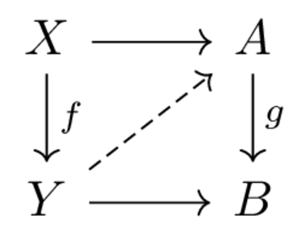
Given a class S of morphisms in \mathcal {C}, let LLP(S) be the class of morphism with the left lifting property with respect to _all_ morphisms f \in S, analogously RLP(S).
It is again not hard to see that RLP and LLP form a Galois connection from the collection of subclasses of morphisms in \mathcal {C} to itself. What is the closure operator LLP(RLP(-))? This is probably a bit harder to motivate than the previous examples, but understanding it is important in model category theory.
As before, we can try to find some constructions that LLP(RLP(-)) is certainly closed under:
- Pushouts, in the sense that if f: X \to Y is in LLP(RLP(-)), and g: X \to Z is any morphism, the induced Z \to X+_Y Z is also in there. - Retracts: given a commutative diagram
where the horizontal composites are identities, if f is in the class, so is g
- Transfinite composition: given a sequence X_0 \to X_1 \to \dots with each map in the class, the maps to the colimit \operatorname {colim}_i X_i are also in the class (here this diagram can be indexed by any ordinal).
Each of these proofs is essentially by a diagram chase.
A class closed under all these constructions is called _saturated_. Then we have _Quillen's Nullstellensatz_ (which is confusingly usually called the _Small object argument_): If \mathcal {C} is locally presentable, and S is a small set, then LLP(RLP(S)) is the smallest saturated class containing S.
I guess you can actually dispense with the function symbols if you want
Demystifying the second law of thermodynamics [demystifying-the-second-law-of-thermodynamics]
- November 22, 2020
-
Eigil Fjeldgren Rischel
Demystifying the second law of thermodynamics [demystifying-the-second-law-of-thermodynamics]
- November 22, 2020
- Eigil Fjeldgren Rischel
Thermodynamics is really weird. Most people have probably encountered a bad explanation of the basics at some point in school, but probably don't remember more than
- Energy is conserved
- Entropy increases
- There's something called the ideal gas law/ideal gas equation.
Energy conservation is not very mysterious. Apart from some weirdness around defining energy in general, it's just a thing you can prove from whatever laws of motion you're using.
But _entropy_ is very weird. You've heard that it measures "disorder" in some vague sense. Maybe you've heard that it's connected to the Shannon entropy of a probability distribution H(p) = \sum _x - p(x)\ln p(x). Probably the weirdest thing about it is the law it obeys: It's not conserved, but rather it _increases_ with time. This is more or less the only law like that in physics.
It gets even weirder when you consider that at least classical Newtonian physics is _time-symmetric_. Roughly speaking, this means if you have a movie of things interacting under the laws of Newton, and you play it backwards, they're still obeying the laws of Newton. An orbiting moon just looks like it's orbiting in the other direction, which is perfectly consistent. A stone which is falling towards earth and accelerating looks like it's flying away from earth and decelerating - exactly as gravity is supposed to do.
But if there's some "entropy" quality out there that only increases, then that's obviously impossible! When you played the movie backwards, you'd be able to tell that entropy was decreasing, and if entropy always increases, some law is being violated. So what, is entropy some artefact of quantum mechanics? No, as it turns out. Entropy is an artefact of the fact that you can't measure all the particles in the universe at once. And the fact that it seems to always increase is a consequence of the fact that matter is stable at large scales.
The points in this post are largely from E.T. Jaynes' Macroscopic Prediction.
A proof that entropy doesn't always increase
- November 22, 2020
-
Eigil Fjeldgren Rischel
A proof that entropy doesn't always increase
- November 22, 2020
- Eigil Fjeldgren Rischel
Let X be the set of states of some physical system. Here I will assume that there is a finite number of states and time advances in discrete steps - there is some function T: X \to X which steps time forward one step. We assume that these dynamics are time-reversible in the weak sense that T is a bijection - every state is the future of exactly one "past" state. Let S: X \to \mathbb {R} be some function. Assume S(x) \leq S(Tx) - in other words, S can never decrease. Then S is constant, i.e S(x) = S(Tx).
Proof: Assume for contradiction S(x) < S(Tx) for some x. Since X is finite, let \sum _x S(x) be the sum of S over all states. Then clearly \sum _x S(x) = \sum _x S(Tx), since Tx just ranges over all the xs. But on the other hand, we have S(x) \leq S(Tx) for all x, and S(x) < S(Tx) in at least one case. So we must have \sum _x S(x) < \sum _x S(Tx) - contradiction.
This proof can be generalized to the continuous time and space case without too much trouble, for the types of dynamics that actually show up in physics (using Liouville's Theorem). The proof above still requires a _bounded_ phase volume (corresponding to the finiteness of X). To generalize to other situations we need some more assumptions - the easiest thing is to assume that the dynamics are time-reversible in a stronger sense, and that this is compatible with the entropy in some way.
(You can find easy counterexamples in general, e.g. if X=\mathbb {Z} and the dynamics are T(x) = x+1, then obviously we really do have that S(x) =x is increasing. Nothing to do about that.)
Anyways the bounded/finite versions of the theorems do hold for a toy thermodynamic system like particles in a (finite) box - here the phase volume really is bounded.
The true meaning of entropy
- November 22, 2020
-
Eigil Fjeldgren Rischel
The true meaning of entropy
- November 22, 2020
- Eigil Fjeldgren Rischel
Okay, so what the hell is going on? Did your high school physics textbook lie to you about this? Well, yes. But you're probably never going to observe entropy going down in your life, so you can maybe rest easy.
Let X be the physical system under consideration again. But suppose now that we can't observe x \in X, but only some "high-level description p(x) \in Y. Maybe x is the total microscopic state of every particle in a cloud of gas - their position and momentum - while p(x) is just the average energy of the particles (roughly corresponding to the temperature). x is called a _microstate_ and y = p(x) is called a _macrostate_. Then the _entropy_ of y \in Y is S(y) = \ln (p^{-1}(\{y\})) - the logarithm of the number of microstates x where p(x) = y. We say these are the microstates that _realize_ the macrostate y.
The connection with Shannon entropy is now that this is exactly the Shannon entropy of the uniform distribution over p^{-1}(y). This is the distribution you should have over microstates if you know nothing except the microstate. In other words, the entropy measures your uncertainty about the microstate given that you know nothing except the macrostate.
There are more sophisticated versions of this definition in general, to account for the fact that
- In general, your microstates are probably sets of real numbers, and there are probably infinitely many compatible with the macrostate, so we need a notion of "continuous entropy" (usually called differential entropy, I think) - Your measurement of the macrostate is probably not that certain (but this turns out to matter surprisingly little for thermodynamic systems),
but this is the basic gist.
Why entropy usually goes up
- November 22, 2020
-
Eigil Fjeldgren Rischel
Why entropy usually goes up
- November 22, 2020
- Eigil Fjeldgren Rischel
Okay, so why does entropy go up? _Because there are more high-entropy states than low-entropy states_. That's what entropy _means_. If you don't know anything about what's gonna happen to x (in reality, you usually understand the dynamics T themselves, but have absolutely no information about x except the macrostate), it's more likely that it will transfer to a macrostate with a higher number of representatives than to one with a low number of representatives.
This also lets us defuse our paradox from above. In reality, entropy doesn't go down for literally every microstate x. It's not true that S(p(Tx)) > S(p(x)) for all x - I proved that impossible above. What _can_ be true is this: given a certain macrostate, it's more probable that entropy increases than that it decreases.
We can consider an extreme example where we have two macrostates L and H, corresponding to low and high entropy. Clearly the number of low-entropy states that go to a high-entropy state is exactly the same as the number of high-entropy states that go to a low-entropy state. That's combinatorics. But the _fraction_ of low-entropy states that go to high-entropy is then necessarily larger than the fraction of high-entropy states that go to low-entropy states.
In other words, P(H(x_{t+1})|L(x_t)) > P(L(x_{t+1})|H(x_t))
Why entropy (almost) always goes up
- November 22, 2020
-
Eigil Fjeldgren Rischel
Why entropy (almost) always goes up
- November 22, 2020
- Eigil Fjeldgren Rischel
Okay, but that's a lot weaker than "entropy always increases"! How do we get from here to there? I could say some handwavy stuff here about how the properties of thermodynamic systems mean that the differences in the number of representatives between high-entropy and low-entropy states are massive - and that means the right-hand probability above can't possibly be non-neglible. And that in general this works out so that entropy is almost guaranteed to increase.
But that's very unsatisfying. It just happened to work out that way? I have a much more satisfying answer: entropy almost always increases because matter is stable at large scales.
Wait, what? What does that mean?
By "matter is stable at large scales", I mean that the macroscopic behaviour of matter is predictable only from macroscopic observations. When a bricklayer builds a house, they don't first go over them with a microscope to make sure the microstate of the brick isn't going to surprise us later. And as long as we know the temperature and pressure of a gas, we can pretty much predict what will happen if we compress it with a piston.
What this means is that, if p(x) = p(x'), then _with extremely high probability_, p(Tx) = p(Tx'). It might not be literally certain, but it's sure enough.
Now, let's say we're in the macrostate y. Then there is some macrostate y' which is _extremely likely_ to be the next one. For very nearly all x so that p(x) = y, we have p(Tx) = y'. But this means that y' must have at least that many microstates representing it, since T is a bijection. So the entropy of y' can at most be a _tiny_ bit smaller than the entropy of y - this difference would be as tiny as the fraction of x with p(Tx) \neq y', so we can ignore it.
So unless something super unlikely happens and p(Tx) \neq y', entropy goes up.
By the way, this also explains what goes wrong with time-reversibility, and why in reality, you can easily tell that a video is going backwards. The "highly probably dynamics" Y \to Y, which takes each macrostate the the most probable next state, don't have to be time-reversible. For instance, let's return to the two-macrostate system above. Suppose that with 100% certainty, low-entropy states become high-entropy. Let there be N_L low-entropy states and N_H high-entropy states. Then, just because T is a bijection, there must be N_L high-entropy states that become low-entropy. Now if N_H \gg N_L, then practically all high-entropy states go to other high-entropy states. So L \mapsto H but H \mapsto H.
Of course in reality, if you start with a low-entropy state and watch this unfold for a _really_ long time, you'll eventually see it become a low-entropy state again. It's just extremely unlikely to happen in a short amount of time.
Entropy is not exactly your uncertainty about the microstate
- November 22, 2020
-
Eigil Fjeldgren Rischel
Entropy is not exactly your uncertainty about the microstate
- November 22, 2020
- Eigil Fjeldgren Rischel
The entropy of a given macrostate is the uncertainty about the microstate _of an observer who knows only the macrostate_. In general, you have more information than this. For example, if the system starts in a low-entropy state, and you let it evolve into a high-entropy state, you know that the system is in one of the very small number of high-entropy states which come from low-entropy states! But since you can only interact with the system on macroscales, this information won't be useful.
A response to Maudlin on credence and chance [a-response-to-maudlin-on-credence-and-chance]
- November 18, 2020
-
Eigil Fjeldgren Rischel
A response to Maudlin on credence and chance [a-response-to-maudlin-on-credence-and-chance]
- November 18, 2020
- Eigil Fjeldgren Rischel
Credence - and chance - without numbers (and with the Euclidean property) is a philosophy paper by Tim Maudlin. In it, Maudlin discusses the closely related notions of _credence_, the subjective likelyhood that a specific agent associates to some outcome, and _chance_, the objective likelyhood that the event happens. He argues that
- The traditional approach of measuring these outcomes with numbers is wrong, but
- this shouldn't trouble us too much, because we can do a lot without them.
As it happens, I have my own serious reservations about the traditional measure-theoretic formulation of probability (due to Kolmogoro). By I still think this paper is more or less terrible. Maudlin displays a Wikipedia-level understanding of the paradoxes surrounding infinity in probability theory. His proposed solution amounts to enumerating a list of properties that an agent's system of credence should satisfy, and arguing that these axioms suffice for the things we usually want to do with "subjective degree of belief". This is actually fine such as it is, but his description of this is also seriously lacking.
Infinity in probability theory
- November 18, 2020
-
Eigil Fjeldgren Rischel
Infinity in probability theory
- November 18, 2020
- Eigil Fjeldgren Rischel
There's the following very classical paradox in probability theory: Suppose you toss a dart at a dartboard. For each point p on the dartboard, we can ask for the probability that the dart hits that exact point p. Suppose we have no relevant information about the tossing process, so that each point seems equally likely. What is the probability P(p)? Well, it can't be more than zero, because then the total probability, the probability that the dart hits any point, would be, not just greater than 1, but infinite! This is because there are infinitely many points on the dartboard, and any positive number added to itself infinitely many times is infinite. But hold on, it also can't be 0, because that means by a similar argument that the probability that the dart hits any point on the dartboard is also 0 - but it must hit _some_ point.
First I'll note that this problem actually is _not_ entirely resolved by measure theory. Measure theory allows for a uniform probability measure on continuous spaces like the interval [0,1] (by, essentially, not allowing us to add probabilities up in every case. More on this later). But if we just suppose a countable dartboard, we're left with the same problem.
But, hang on, does a dartboard really have an infinite number of points? And what does it mean for the dart to hit a point? Certainly the point of the dart _itself_ has a non-infinitesimal area, so that if we partition the dartboard into "points" of that size, there will be a finite number, each of which we can assign some positive probability without issue. In general, any area on the dartboard, no matter how small, has a positive probability of being struck by the dart, and this remains true no matter how small we make the dart, as well.
In other words, this paradox hinges on an infinitesimal dart, as well as an infinitesimally accurate measuring tape with which to measure the coordinates, which presumably has infinitely long numerals on it (presumably the person assigning these credences has an infinitely large brain as well, to be able to hold in their minds the coordinates pointing out a specific point on the dartboard to infinite precision).
Any mathematician knows that you have to handle a situation like this _very carefully_. You cannot expect to apply your intuition directly and get consistent results. I am actually kind of surprised to find serious philosophers making this kind of argument in 2020. This is on par with saying that Zeno's paradox proves you can't use numbers to measure space (or time).
To be fair to Maudlin here, I do think he has a point: there do seem to be situations where you should be indifferent between a (countably) infinite number of outcomes, and probability theory won't let you do that. Dartboards is just a bad example.
Maudlin's shaky relationship with infinity shows up again in his discussion of the classical Kolmogorov approach to probability. He cites the definition of a _finitely additive_ probability measure, and not the \sigma -additive (or countably additive) version used by every probability theorist and statistician in the world. Then he criticizes it for only being finitely additive!
He also critizises the use of a \sigma -algebra, arguing that it seems irrational to exclude certain sets from consideration. I think Maudlin needs to spend a small amount of time understanding non-measurable sets before arguing they're stupid. For one thing, a nonmeasurable subset of \mathbb {R}^2 (such as we might ask "will the dart hit a point in this subset or not" of), is _extremely weird_. It's consistent with ZF minus Choice that there exist no such sets. Certainly such sets always contain regions of "infinite complexity", in the sense that there are (non-infinitesimal) regions of the dartboard so that, if the dart hits there, no finite amount of measurement will suffice to determine whether it is in the set or out of it. Indeed, it's not too far off the mark to think of the \sigma -algebra as denoting the "determinable" events.
The fact that a probability measure is only _countably_ additive is still a bit weird. You can make philosophical arguments for this choice: To check whether a \in \cup _n A_n, we can check whether a \in A_n for each a - and this is guaranteed to give you an answer in a finite amount of time, but only if you're taking a finite union. There are reasonable counterarguments to this, but Maudlin doesn't engage with this topic at all - it really seems as if he doesn't realize that mathematicians have been taking infinite disjunctions of events all this time[^fn:1].
Maudlin's solution
- November 18, 2020
-
Eigil Fjeldgren Rischel
Maudlin's solution
- November 18, 2020
- Eigil Fjeldgren Rischel
Maudlin's proposed replacement for numbers is essentially the following idea: it's not required that a person's credences be represented by some definite "thing" - a number or another mathematical object. Instead we should ask about the _structure_ on the system of credences, and what rules this should follow for any "rational" person.
This is actually a very good idea! Structuralism! Defining things extrinsically rather than intrinsically! I like this approach.
Let's go over the basic principles that Maudlin comes up with. The paper is short on rigor, but since it's a philosophy paper and not a math paper, I won't hold that against it.
- The set of "credences" should have a partial order[^fn:2]. - The map \operatorname {Cr} which assigns an event its credence should be order-preserving - in other words, if event P entails the event Q, then \operatorname {Cr}(P) \leq \operatorname {Cr}(Q). - There should be a least credence \bot and a greatest credence \top , corresponding respectively to the credence in an event which is certain not to happen or certain to happen (say, a contradiction and a tautology). - The map \mathrm {Cr} should have the following property: if P \Rightarrow Q, \operatorname {Cr}(P) = \operatorname {Cr}(Q),
then \operatorname {Cr}(Q \wedge \neg P) = \bot . This is the so-called "Euclidean property" that Maudlin cannot stop going on about: "the whole is greater than the part", or in this case, if P entails Q, and it's possible that Q but not P (i.e. Q does not entail P), then our credence in Q must be _strictly greater_ than our credence in P.
We can define a partial addition operation on credences, denoted \oplus in the paper, by setting \operatorname {Cr}(P) \oplus \operatorname {Cr}(Q) = \operatorname {Cr}(P \vee Q) whenever \Cr (P \wedge Q) = \bot . It's not exactly clear in the paper whether we extend this using the equality on credences - for example, whether we can assign a value to \operatorname {Cr}(P) \oplus \operatorname {Cr}(P) by finding some other event Q so that \operatorname {Cr}(P) = \operatorname {Cr}(Q), \operatorname {Cr}(P \wedge Q) = \bot , and setting \operatorname {Cr}(P) \oplus \operatorname {Cr}(P) = \operatorname {Cr}(P \vee Q). This seems a harmless enough extension (if we really regard credences as _equal_, and not just equivalent in some sense, it seems inevitable), but Maudlin doesn't really spell it out. Nevertheless the addition is still _partial_, since, for example, when rolling a fair dice, we can't add our credence in the event "The result will be one of 1,2,3,4" to itself, since there is no mutually exclusive event which is equally likely. This is not really a bug - indeed, while you can add probabilities and get a number greater than 1, you can't really treat that number _as a probability_.
So far, Maudlin's approach differs from the Kolmogorovian approach chiefly in that he lets the poset of credences be any ordered set, not just numbers, and that he doesn't require the order on credences to be _total_ - we can have no opinion about the relative plausibility of two events without declaring them _equally_ plausible. This is reasonable enough. Probably the weirdest thing here is that the "Euclidean property" is _also satisfied by Kolmogorov probability!_ The reason that adding a point to a set doesn't change the probability that the dart will land there is simply that it's impossible that the dart will land at that precise point. This is obviously counterintuitive (and there are ways of defending it, and counterarguments to those, and so on - but Maudlin does not engage with this at all), but that is the classical approach. It does not seem to violate the Euclidean property at all.
Having the addition in hand, we can actually reformulate the Euclidean property simply as "\oplus is cancellative", i.e if C \oplus D= C \oplus D' then D = D'. This means that \operatorname {Cr}(Q) = \operatorname {Cr}(P) \oplus \operatorname {Cr}(Q \wedge \neg P), and if this equals \operatorname {Cr}(Q) then \operatorname {Cr}(Q \wedge \neg P) = \bot , since \bot is the unit of addition.
Now Maudlin wants to talk about _relations_ between credences. First of all I have to go on a rant about his whole discussion about ratios. Mathematics has come a long way since Euclid, and citing him like you actually believe his axioms provide a sound formal basis of geometry is not gonna convince anyone that you know what you're talking about. Maudlin goes oddly pedantic and says that the ratio of a circle's circumference to its diameter is not \pi , but rather, the ratio of the number \pi to the number 1, and this is in general what people mean when they identify a ratio with a number. I'm glad to hear that Maudlin has found a solution to the long-standing problem of the identity of mathematical objects (presumably resolving it in favor of a _very_ strong form of Platonism?), but I couldn't find this in the bibliography of the paper or any of his other work. Until I do, I have to insist that "loose talk" is when you insist that two mathematical objects identified under isomorphism cannot possibly be called equal, not the other way around.
Okay, rant done. We can define the ratios between credences by addition. For example, we can say that credence C is twice as big as credence D if C = D \oplus D. Maudlin, quoting Euclid: "Magnitudes are said to have a ratio to one another which can, when multiplied, exceed one another". There is however a serious problem with this: the partiality of addition means that you can't _compare_ these ratios, and many pairs of credences have no ratio to one another, even though Maudlin insists that they do.
Let's pull back here a bit. Suppose I have an ordered (commutative) monoid (M,\leq ,+). Then I can say that m,m' have a ratio to each other if there exist n,n' \in \mathbb {N} so that n.m \geq m', and n'.n' \geq m. If this is true, we can actually obtain a unique real-numbered ratio "m/m'" as the supremum of all n/n' \in \mathbb {Q} so that n.m' \leq n'.m.[^fn:3] Here I'm using n.m to denote the n-fold sum m + m + \cdots + m.
Now, this _doesn't_ work for credences - even in situations where it feels like it should[^fn:4]. The increasingly accurate rational approximations to the "true" real ratio requires longer and longer chains of addition, but this is generally impossible to define for credences. We can define what it means for C/C' to be an integer - namely that n.C' = C. We can also _sometimes_ define what it means for C/C' to be a rational number - for example if 2.C = 3.C', we can say C/C' = 2/3. But if e.g. C = \top , there's no way to make this work. And, crucially, we can't usually compare ratios with each other either - otherwise, we might have argued that expecting number representations for each ratio is too much.
As it stands, by Maudlin's (or rather, Euclid's) definition of ratio, there is no ratio between \top and any event with "probability greater than 1/2" (speaking informally - of course credences aren't probabilities and so on), in contrast with how Maudlin uses it.
This is an area where the paper could really have benefited from some rigor. It's not clear whether Maudlin means to tack on "ratios" as a primitive notion - so that, in addition to having a "more likely than" relation on credences, we have ratios between certain pairs of credences, which can be compared.
All these issues could be solved _very easily_, by imposing some extra structure on the model. For instance we could add "formal sums" of credences which don't have a sum, and say that the statement 2.P \geq Q makes sense even when 2.P is not defined as a credence.
Closing
- November 18, 2020
-
Eigil Fjeldgren Rischel
Closing
- November 18, 2020
- Eigil Fjeldgren Rischel
As I mentioned above, I actually, genuinely think it's a good idea to think about replacements for classical probability theory. In some sense my own work on Markov categories is a version of this, a sort of "synthetic probability theory". Much like Maudlin, Markov categories start by asking "what structure do we actually need to do the job of probabilities?". They go in a very different direction, not least because we actually care about the job that probabilities do for people in the real world, but the spirit is actually similar.
But stress-testing your theory by applying it to situations involving infinity - without working rigorously with infinity _at all_ - is bound to get you into trouble. Frankly, if the only problem your theory solves is that it makes sense of infinite conjunctions, it's basically useless. Infinite conjunctions only come up in abstrac mathematical models, and trust me, those guys aren't really looking for a new theory. In the real world, it's very hard to write down infinitely many statements and think about your credence in the statement "one of these is true".
The mathematical idea in this paper - which, again, I actually don't think is a stupid idea - could have fit in a couple of pagers, including a fair amount of exposition and the easy fixes to the problem mentioned above. The philosophical work here seems mainly to be a takedown of traditional probability, which falls woefully flat.
[^fn:1]: A less elegant reason for asking for countable composition but not general infinitary composition is that it leads to a useful, theoretically convenient theory, but still allows for measures like the uniform measure on the interval. This is just an argument from practicality - we take these axioms instead of some others because they make the calculations work out - so I won't hold it against Maudlin if he doesn't take this argument very seriously [^fn:2]: Maudlin seems to not know this term, which probably could have cut several pages from his exposition [^fn:3]: Ironically, in the usual construction of real numbers, they are limits of ratios (between integers), so one could make a convincing argument that a real number really is literally a ratio. [^fn:4]: Credences can be "infintesimal, in the sense that we might have n.C \leq C' for ALL n. That's not what I'm talking about."
reMarkable 2 review [remarkable-2-review]
- November 10, 2020
-
Eigil Fjeldgren Rischel
reMarkable 2 review [remarkable-2-review]
- November 10, 2020
- Eigil Fjeldgren Rischel
I recently got a reMarkable 2. I've had it for one week. This is my review of it so far.
TLDR
- November 10, 2020
-
Eigil Fjeldgren Rischel
TLDR
- November 10, 2020
- Eigil Fjeldgren Rischel
- It's very very good and I'm happy I bought one. If your relationship with working "on things" is like mine, I recommend it. - It's expensive and you can get an iPad + accessories + Apple Pencil for the same price, which may be better - There are some annoyances
Would I buy the reMarkable again? That is, if it was struck by a meteor tomorrow, would I buy a new one? Yes (but see my notes on other options). In my opinion, these devices are now good enough that it's worth paying a premium to get the "paper experience". I would not recommend saving up for the reMarkable - that is, if your disposable income is small and you'd need to make an effort over a time period to find the money, it's probably not worth it. If you own a laptop and are considering buying a tablet, which you anticipate using largely for reading and writing, the reMarkable is recommendable. If you're in the market for a tablet to use also for laptop tasks, it's not up to the job.
Paper and Me
- November 10, 2020
-
Eigil Fjeldgren Rischel
Paper and Me
- November 10, 2020
- Eigil Fjeldgren Rischel
My fiancé is one of those stationery nerds. She own several different fountain pens and a metric boatload of ballpoint pens, gel pens, highlighters, markers, and what have you. She buys a specific brand of Japanese calendar (Hobonichi) each year. She has had the same color-coding system for her notes since we started university [^fn:1]. She meticulously pagemarks and sorts all her notes into plastic sleeves and binders.
I am not like my fiancé. My workflow for most of my first five years at university consisted of the following:
- Keep a stack of papers and ballpoint pens in my backpack (along with the books I'm using and my laptop and so on). - When you sit down to work somewhere, get laptop, stack of papers, and a ballpoint pen out. - When you need to think, locate a blank spot on a piece of paper in front of you and write there. - If there's no space, go through the papers until you find some space. - When you stop working, gather all the papers into your backpack. - Periodically go through your papers and throw out any that have writing all over them - Periodically add a fresh dump of blank papers to your backpack.
The two points I want to make here is:
- I am a very disorganized person - I fucking love paper
Paper is awesome. I am long paper. Whoever you are, you should be using more paper. There's absolutely no reason to strain your head to the breaking point, keeping a bunch of things inside it, instead of putting them on paper. Actually, if you take one recommendation from this review, just make sure to keep paper and pen wherever you work and use it all the time. Go to these links to buy some _right now_, they're cheap (but you probably have this stuff already - use it!). See also Paper Trauma. I also invite you to consider buying a big notebook, but I haven't tried that yet myself.
But paper has some limitations:
- You sometimes run out - If you want to write your notes about something you're reading on paper, the best place is the thing you're reading - but this requires that it be on paper (instead of a computer). This means you have to buy a book (these have a tendency to pile up rapidly, if it even is a book you can buy) or print it out (this tends to be messy, and you might not have a printer. Back at the university of Copenhagen, I used to print out a lot of stuff and spiral-back it, but I can't do this any more). - Sometimes you lose your old paper where you wrote something important (usually, because you didn't know at the time it would be important). - It's easy to make a mess by creating a huge stack of paper. If you're like me, "clean up your big pile of papers" can sometimes become a bit of an "ugh" task that you can't get around to and which sucks up a lot of energy.
Enter the reMarkable 2. A "next-generation paper tablet", it promises you that you can "Replace your notebooks and printed documents with the only tablet that feels like paper". Naturally, I was intrigued.
General experience and thoughts
- November 10, 2020
-
Eigil Fjeldgren Rischel
General experience and thoughts
- November 10, 2020
- Eigil Fjeldgren Rischel
The writing experience is _very very good_. It doesn't quite feel like paper - it's not _that_ close - but apart from actually writing on paper it's the best I've tried (having, admittedly, not tried that many). It's leagues ahead of writing on a "normal" tablet using a stylus.
Drawing on the reMarkable has the following advantages over paper:
- You can erase things, perfectly - You can undo/redo strokes - You can zoom - You can select and move things - There's layers, like in image editing software.
The surface feels a bit too smooth - it doesn't have the same friction as dragging a pen over paper. It's still better than a normal screen (like a iPad) though. You can tell they added some texture to make this more lifelike, but it's not the same.
Not surprisingly, it's a bit awkward to hold the tablet with one hand and write with the other. The holding hand doesn't provide quite enough support. You really need to support it with a table or your knees or something.
Probably the biggest thing I would like is a bigger screen.
Notes about the OS
- November 10, 2020
-
Eigil Fjeldgren Rischel
Notes about the OS
- November 10, 2020
- Eigil Fjeldgren Rischel
The "OS", as it is, is basically just a folder structure where you can arrange pdfs, EPUBs (I haven't tried this), and "notebooks", which are basically collections of pages of your drawing/writing/scribbling. You can also add things to "favorites" and sort by "type" (notebook/pdf/EPUB). It's not amazing, especially since it's a bit sluggish to use, but it does the job.
You can get stuff out of and into the reMarkable in a few ways:
- If you create an account in their server and connect it, it automatically syncs to their cloud, and you can get at this data from a desktop app and a mobile app. These are also how you get stuff into it. The syncing here is pretty slow, so I don't use this a lot. - You can send a mail from the tablet with a collection of pages - either annotated pdf/epub or raw notebook. This is what I do, and it works great! - There's also a browser extension which turns a website into an EPUB and sends it to the tablet. It works okay, about the same as something like Pocket or Instapaper. - You can also have the reMarkable convert you handwriting into text and send it as an email. This is actually surprisingly (to me) good, but probably not quite good enough to send a mail without proofreading (you can check and edit the message on the tablet before sending). The first line in the following picture was converted without error, while the second became "The Quick brown tote jumps over the lazy chef".
I haven't tested this extensively, and I expect it to do worse on other languages than English (you can switch the language used in the setting menu).
The physical feel of things
- November 10, 2020
-
Eigil Fjeldgren Rischel
The physical feel of things
- November 10, 2020
- Eigil Fjeldgren Rischel
The pen weighs 19g, and feels about like an ordinary ballpoint pen/fineliner in the hand. I would have liked a bit more weight, but it's not a big deal.
The tablet is pretty light. Holding it in one hand is a bit heavy for me - not TOO heavy to use like that, but I probably won't read like that for, say, multiple hours. This is not a big deal though.
The "Book Folio" cover is fine. It's fairly basic, certainly not "worth" 100 EUR - if there was a market for accesories, you could certainly buy a better one much cheaper. It essentially consists of two pieces of sturdy cardboard (I think), covered on the outside by light grey fabric and on the inside by something that feels like felt. The tablet attached to the backside by magnets - these are not that strong, but they do the job. The pen simply attached to the tablet itself by magnets - again, these do the job, but I would have liked them to be a bit stronger. I am slightly worried about the pen falling off in a bag full of mess and getting into trouble. The front piece also attaches by (weaker) magnets when closed, so it doesn't open by itself.
Notes about my "workflow"
- November 10, 2020
-
Eigil Fjeldgren Rischel
Notes about my "workflow"
- November 10, 2020
- Eigil Fjeldgren Rischel
The basic things I've done with the reMarkable so far breaks down into roughly three categories:
- During video meetings, I've scratched notes on the tablet - I've put things on the tablet to read, and scribbled in the margins while I did so - I've used the blank pages (notebooks) to work on.
Meeting notes
- November 10, 2020
-
Eigil Fjeldgren Rischel
Meeting notes
- November 10, 2020
- Eigil Fjeldgren Rischel
The device doesn't really shine here. The only advantage it has over writing on the computer is that I can keep the window with people's faces visible while writing, which I could do anyway if I had a second monitor. There's something nice about paper writing - maybe the flexibility of not being limited to one line after the other? Maybe something physical? That this captures but writing on the computer doesn't, though. But this is a small advantage.
Reading and scribbling
- November 10, 2020
-
Eigil Fjeldgren Rischel
Reading and scribbling
- November 10, 2020
- Eigil Fjeldgren Rischel
This is the real killer app for me. As noted above, you can put your pdfs on the reMarkable and read them. And while reading them, you can scribble on them. I am one of those people who likes to constantly doodle on things, so the eraser really comes in handy here - I can make a scribble, then erase it, so the margins don't get covered in random noise. This is an advantage I hadn't thought of.
After scribbling and highlighting and so on, I usually send annotated pages to my email. Then they can become part of my diginal notes.
I think the fact that this doesn't browse the internet is probably a huge advantage, because it adds a bit of friction to checking twitter, making me distract myself less. Just having a pdf reader that can't check twitter might contribute a huge amount of value.
Working on blank paper
- November 10, 2020
-
Eigil Fjeldgren Rischel
Working on blank paper
- November 10, 2020
- Eigil Fjeldgren Rischel
As mentioned above, using blank paper to think on is really important to me. On the reMarkable, there's a distinguished "quick pages" notebook with a permanent shortcut to it on the top. This gives you an infinite supply of blank pages to work on. I also use a few other notebooks to collect thoughts about various projects, but this is not very well-organized. The biggest drawback here is that the pages are not very large. I think the screen is slightly broader than A6 format (checked by holding up a folded sheet of A4). This is not optimal - I would like to be able to draw bigger things, to keep more thoughts on the page at once. The jury is still out, but I can't imagine the reMarkable will permanently replace paper in this domain for me - at best, it will supplement it.
Notes on price & comparison to other products
- November 10, 2020
-
Eigil Fjeldgren Rischel
Notes on price & comparison to other products
- November 10, 2020
- Eigil Fjeldgren Rischel
The reMarkable 2 device itself costs 400 EUR (473 USD at current rates, but prices may differ by region). This price point is severely misleading, since it's more or less useless unless you buy a pen (you can read on it, of course, but if that's all you want to do I would definitely consider it overpriced).
The basic "Marker" costs 60 EUR, and the "Marker plus" costs 100 EUR. The only difference is that the plus weighs slightly more and that you can use the rear end to erase. It's probably best to just consider the base price of the device 460 EUR and ask whether you want to pay 40 EUR for the eraser.
Lastly, you can purchase a cover, or "folio". Here your options are the basic folio for 80 EUR, which is simply a sleeve that you can slide the reMarkable into, and the "Book Folio", which is essentially a folder, which magnetically attaches to the back of the reMarkable and wraps around it. This costs 100 EUR for the basic "polymer weave", and 150 EUR for the black or brown "Premium Leather" version. These are "overpriced" in the sense that, if there was a market for reMarkable accessories, you would certainly be able to buy much better protective covers for much less. But there isn't, so you're stuck with these, and the question is whether they're worth the money.
You can also buy a reMarkable 1 with basic Folio and (non-eraser) Marker for 349 EUR.
When I bought my reMarkable, I paid a reduced price because I was buying it early. I bought the Marker Pro and the Polymer Weave Book Folio, and ended up paying 460 EUR.
So how much does the reMarkable 2 cost? Based on my experience so far, the built-in eraser is super convenient and well worth the money. You probably want _some_ sort of protective cover, to prevent the screen from getting dings and scratches, but I have to stress that the Folios really seem to be nothing special. If I was buying it again I would probably buy the Book Folio again, just because 20 EUR isn't a lot and it seems a bit incovenient to be taking it in and out of the sleeve all the time. On that basis, it costs 600 EUR, or ~710 USD.
That's a lot. For that money you could buy an iPad (329 USD), Apple Pencil ($129), and a smart cover ($50), and still have money left over. You could use that money to buy extra memory for the iPad, cellular web access (not a killer app for me, but the reMarkable lacks it). You could even buy an iPad Air, if you maybe skimped out on the cover. I didn't look into the Android options, but presumably those are even cheaper. So if you're looking for a "general work tablet", you should probably skip the reMarkable. If you're looking for the paper feeling, you could consider Paperlike, for just 40 USD (which I have not tried and cannot opine on).
reMarkable really has nothing in the way of tablet features. You can't install any apps (actually, there's a small community of hackers, but nobody is seriously developing third-party software). You wouldn't want to install any of the apps you have on other devices even if you could, because the refresh speed is too low for most "normal" software to really be usable. You can't browse the internet.
What you can do is basically:
- Write and draw with a stylus like you were drawing on blank paper - Read pdfs and ebooks, and write on them.
If stuff like that is such an important part of your workflow that getting a significantly better experience than you would doing the same thing on an iPad is worth giving up _all of the iPad's other features_, you should consider the reMarkable. Personally, this is basically the only reason I would really want to own a tablet anyway. In fact, the fact that I can't browse the internet on it is probably a strong feature in its favor, since it makes it harder to distract yourself with twitter.
Another comparison is with the line of products from Boox. The most direct comparison is with the Note Air, which has a similar form factor and price point. There is also Supernote. I have no experience with any of these. It seems that the Boox Note Air is generally more feature-rich than the reMarkable - it actually runs Android, and is thus closer to a "proper" tablet. This review may provide some information, and recommends the Note Air.
I have to say these products are really tempting me, especially the ones with larger screens. If I was buying a new "paper tablet" today, I would seriously consider them.
[^fn:1]: for the record, her opinion of my reMarkable was that it seemed awesome, but it was a nonstarter for her, because it didn't do colors
Euler's method is compositional [eulers-method-is-compositional]
- November 4, 2020
-
Eigil Fjeldgren Rischel
Euler's method is compositional [eulers-method-is-compositional]
- November 4, 2020
- Eigil Fjeldgren Rischel
Another day, another post about dynamical systems. Today, I want to think about _open_ dynamical systems. You can think of an open dynamical system as a system where
- The dynamics are parameterized by some variable (which is supposed to vary with time)
- And some function of the state is exposed (maybe to parameterize other systems).
I want to describe two types of open dynamical systems: continuous ones and discrete ones, and show that Euler's method is a compositional mapping between them.
Open dynamical systems
- November 4, 2020
-
Eigil Fjeldgren Rischel
Open dynamical systems
- November 4, 2020
- Eigil Fjeldgren Rischel
A _continuous open dynamical system_ consists of the following data:
- An input set \mathbb {R}^I - An output set \mathbb {R}^O - A state set \mathbb {R}^S - A "dynamics" D: \mathbb {R}^{I+S} \to \mathbb {R}^S. - A "readout" r: \mathbb {R}^{S} \to \mathbb {R}^O.
This is a continous open dynamical system I \to O. Here I,O,S are natural numbers. Note that we are constraining our spaces to being \mathbb {R}^n. Of course we could have made sense of the above definition for any smooth manifold, asking instead for a map I \times S \to TS so that for each i the map S \to TS is a section of the tangent bundle. The reason we're looking only at Euclidean spaces is because, to actually use Euler's method, we need a way of "stepping along the derivative". In our case this is given by simply adding the derivative - in general, we need a map TS \to S.
A trajectory of this dynamical system is a pair of functions i(t),s(t) so that s'(t) = D(i(t),s(t)).
Given systems I \to X, X \to O, we can compose them to obtain a system I \to O. Suppose the state, dynamics and readout of the two systems are respectively S_1,D_1,r_1,S_2,D_2,r_2. Then the state of the composed system is S_1 + S_2, the readout is simply (s_1,s_2) \mapsto r_2(s_2), and the dynamics are D(i,s_1,s_2) = (D_1(i,s_1),D_2(r_1(s_1),s_2)). This corresponds to plugging the output of the first system into the input of the second.
Note that this does not form a category, because there are no identities - there is no way to simply feed the input into the output.
Now for the discrete systems: A discrete open dynamical system consists of the following data:
- An input set I - An output set O - A state set S - An update function U: I \times S \to S. - A readout function r: S \to O.
Now the composition is pretty much analogous: given systems (S_1,U_1,r_1): I \to X, (S_2,U_2,r_2) : X \to O, the composite has input I, output O, state space S_1 \times S_2, readout (s_1,s_2) \mapsto r_2(s_2), and update U_2(i,s_1,s_2) = (U_1(i,s_1),U_2(r_1(s_1),s_2)).
Again, there are no identities.
Euler's method
- November 4, 2020
-
Eigil Fjeldgren Rischel
Euler's method
- November 4, 2020
- Eigil Fjeldgren Rischel
Recall that _Euler's method_ is a way of solving a differential equation y' = F(y). Given a starting condition y(0) = y_0, we fix some step size h and move forward one step at a time, approximating y(t + h) \approx y(t) + hy'(t) = y(t) + hF(y(t)).
This is essentially replacing a continuous dynamic system with a discrete dynamical system. The state space is the same, and the update function steps forward h by the above method. Formally, if (I,O,S,D,r) is a continuous dynamical system, define Eu_h(I,O,S,D,r) to have
- State space \mathbb {R}^S - the same state space, essentially. - Input space \mathbb {R}^I - Output space \mathbb {R}^O - Update function U(i,s) = s + hD(i,s) - Readout simply given by r
Then, we have that Eu_h is _compositional_ - in other words, if X,Y are continuous systems and X;Y their composite, then Eu_h(X;Y) = Eu_h(X);Eu_h(Y). The proof is essentially just by writing out the definitions.
- The desired identity for in/output, state sets and readout is clear. - For the update, on the left-hand side the update is given by U(i,s_1,s_2) = (s_1,s_2) + h(D_1(i,s_1),D_2(r_1(s_1),s_2)). On the left-hand side, the update is given by U(i,s_1,s_2) = (s_1 + hD_1(i,s_1), s_2 + hD_2(r_1(s_1),s_2)) - these are of course equal.
Higher-order methods
- November 4, 2020
-
Eigil Fjeldgren Rischel
Higher-order methods
- November 4, 2020
- Eigil Fjeldgren Rischel
In ODE solving, a "higher-order method" is one that tries to incorporate information about higher derivatives to make a better estimate. We can view Euler's method as, essentially, calculating y(t+h) by replacing y with its first-order Taylor approximation T_1y(t+h) = y(t) + hy'(t), which we can calculate from the differential equation. We can often get a better estimate by incorporating higher derivatives - by trying to compute y(t) + hy'(t) + \frac {h^2}{2}y^{(2)}(t), for example. Essentially, we are incorporating information about how the derivative will change (or how we think it will change) over the interval [t,t+h]. If it's going up, then we'll get a higher value than we expected just from looking at the derivative now. If it's going down, we'll get a lower value.
The issue here, of course, is that we can't compute the second derivative directly - the differential equation doesn't tell us what it should be. That leaves us with two options
- Derive both sides of y'(t) = F(y(t)) to get y''(t) = F'(y(t))y'(t) = F'(y(t))F(y(t)).
Of course, this requires that the function F in the equation is actually differentiable, and that you have access to a symbolic representation so that you can compute the derivative explicitly. This falls in the general class of methods called _multiderivative methods_. It's easy to see how the above also gives a mapping from continuous systems to discrete ones, although I have not checked the details of compositionality.
- Estimate y''(t) \approx \frac {y'(t)- y'(t-h)}{h} = \frac {F(y(t)) - F(y(t-h))}{h}. This can then be calculated from the past two steps.
It's not immediately obvious how to make this into a discrete dynamical system. After all, the next state depends not only on the current state, but also on the previous one. The idea will be to make a state of the discrete system consist of _two_ points in the space - the transition replaces the first with the second, and computes a new second point by the method. Explicitly, given as above a continuous dynamical system:
- The input and output are as Euler's method - The state is \mathbb {R}^S \times \mathbb {R}^S. - The readout is r(s_1,s_2) = r(s_2) (the readout of the "present") state. - The update is U(i,s_1,s_2) = (s_2, s_2 + hD(i,s_2) + \frac {h}{2}(D(i,s_2) - D(i,s_1)))
Note that in this method, we are updating under the assumption of constant input - it may be more appropriate to remember the last input as well, and use that. In any case, I have not verified compositionality of this method either.
Cofree dynamical systems and chaos [cofree-dynamical-systems-and-chaos]
- October 30, 2020
-
Eigil Fjeldgren Rischel
Cofree dynamical systems and chaos [cofree-dynamical-systems-and-chaos]
- October 30, 2020
- Eigil Fjeldgren Rischel
This blog post largely retraces ideas from Lawvere: Functorial remarks on the general concept of chaos. I saw this in this tweet from Jade Master, which this blog post is basically an extended version of. Hat tip to her.
Let's try to apply category theory to the study of "dynamical systems". What is a dynamical system? There are a lot of different versions:
- A discrete dynamical system is a set S with a map S \to S.
- A discrete Markov process if a countable set S equipped with a stochastic S\times S matrix.
- A smooth dynamical systsem is a smooth manifold M equipped with a section of the tangent bundle M \to TM.
Today, we'll take the following general view:
Let \mathcal {C} be a symmetric monoidal category, and let (T,+,0) be a commutative monoid in \mathcal {C}[^fn:1]. Then a T-dynamical system is simply an object S of \mathcal {C} equipped with an action of T, T \otimes S \to S.
We think of the elements of T as "time-shifts", and the composition adds these together. Using this, we can recover a wide variety of different types of dynamical systems:
- Let \mathcal {C} be the category of sets, equipped with the cartesian monoidal structure. Let T = \mathbb {N}_0. Then a \mathbb {N}_0-dynamical system is exactly a discrete dynamical system in the previous sense.
- Let instead \mathcal {C} = \aleph _0\operatorname {-}\mathsf {Stoch} be the category of countable sets and Markov kernels, and let T be \mathbb {N}_0 again (with the usual monoidal structure regarded as a deterministic Markov kernel). Then a \mathbb {N}_0-dynamical system is exactly a discrete Markov process[^fn:2]
- Let \mathcal {C} be the category of smooth manifolds with the Cartesian monoidal structure, and let T = \mathbb {R}. Then an \mathbb {R}-dynamical system is _almost_ the same thing as a smooth dynamical system in the above sense. A \mathbb {R}-dynamical system picks out a smooth trajectory f(-,m) : \mathbb {R} \to M for each m \in M, in a compatible way. This gives a smooth vector field (i.e a smooth dynamical system in the above sense) m \mapsto f'(0,m).
This is not quite a 1-1 correspondence, for example because even smooth dynamical systems in that sense can experience "finite-time-blowup". For example, if we let M = \mathbb {R}, then this a dynamical system is just an ordinary (time-independent) differential equation. If we put f'(t) = f(t)^2, the unique solution given f(0) = y_0 is \frac {1}{y_0^{-1}-x}, which goes to \infty as x \to y_0^{-1}. So there is no way to find a trajectory, extended for arbitrarily long time, which solves this equation. But on the other hand, perhaps equations like this are bad and shouldn't be counted. Anyways, they are not dynamical systems in this sense.
Let Dyn(T) denote the category of T-dynamical systems - their maps are simply T-equivariant maps. There is an obvious forgetful functor Dyn(T) \to \mathcal {C}.
Suppose \mathcal {C} is a closed monoidal category. Then the above functor has a right adjoint, which sends M to [T,M]. T acts on [T,M] simply by "translation", i.e (t.f)(t') = f(t+t') To be more formal, the map T\otimes [T,M] \to [T,M] is adjoint to the map T \otimes [T,M] \otimes T \to M given by multiplying the 2 Ts, then evaluating the hom.
Proof: We claim that Hom_{Dyn(T)}([M,[T,M']]) \cong Hom_\mathcal {C}(M,M').
Suppose we have a T-equivariant map \phi : M \to [T,M']. T-equivariance, of course, means that the diagram
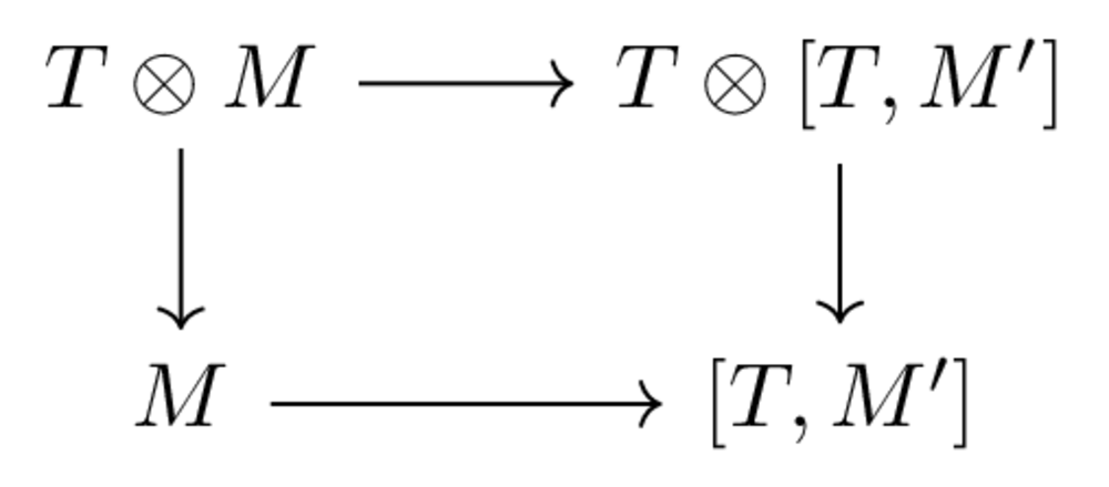
commutes.
The bare map M \to [T,M'] corresponds to a map M \otimes T \to M'. The above commutative square means that this square commutes:
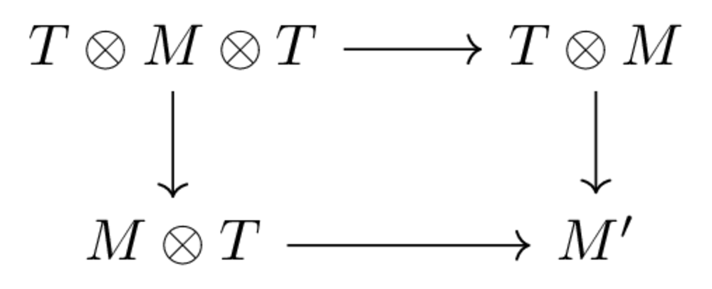
The bottom way around is "let T act on M, then use the map". The other one is "multiply the Ts together, then use the map".
Now let's insert the unit into the right-hand T:
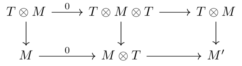
Both these squares commute. And the top arrow is just the identity. In other words the classifying map T \otimes M \to M' must equal the other composite, which is "act, and evaluate at 0". Equationally, if f: M \to [T,M'], this means f(m)(t) = f(t.m)(0). This means the map f:M \to [T,M'] is uniquely determined by the map M \to M' given by evaluation at 0. On the other hand, it's not hard to see that any map M \to M' can be extended to an equivariant map by this method. This concludes the proof.
Now, what can we do with these "cofree dynamical systems"[^fn:3]? Here is a cool thing: We can give a categorical definition of _chaos_.
Let M be a T-dynamical system. Let o:M \to X be a map in \mathcal {C} on the underlying space of M. We can think of o as an "observable": some property of the state which we can measure. There is a corresponding map of systems M \to [T,X] which takes each point in M to its trajectory of observations We say M is _chaotic_ with respect to o if map M \to [T,X] is an epimorphism.
If we think of an epimorphism as a "surjection", this means every possible sequence of observations is possible. In other words, our current observations don't exclude any possible pattern of future observations.
[^fn:1]: It is not really important that these are symmetric and commutative, but I can't be bothered to keep track of the order, and I don't have any natural non-commutative examples [^fn:2]: It may have been more natural to consider finite-state Markov processes, but of course \mathbb {N}_0 isn't finite, so that wouldn't quite have worked [^fn:3]: Incidentally, there is also a further left adjoint, the "free dynamical system", given by M \mapsto T \otimes M
Chu spaces and linear logic [chu-spaces-and-linear-logic]
- October 25, 2020
-
Eigil Fjeldgren Rischel
Chu spaces and linear logic [chu-spaces-and-linear-logic]
- October 25, 2020
- Eigil Fjeldgren Rischel
A _Chu space over S_ consists of a pair of sets (X,U), and a function e: X \times U \to S. A map of chu spaces (X,U,e) \to (Y,V,e') is a pair of maps X \to Y, V \to U so that the diagram
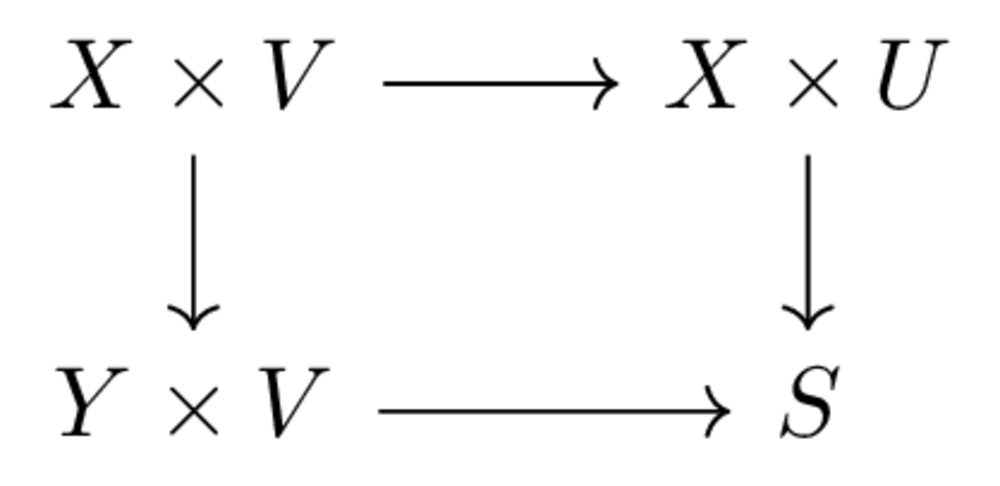
commutes. This defines a category of Chu spaces, called Chu(Set,S) You can think of a Chu space as a normal-form game. X is the set of choices available to one player, and U is the set of choices available to the other. The outcome, given the choices x and u, is e(x,u).
You can think of a map of Chu spaces as a way of transforming strategies between the two games. If you would play x \in X in the original game, you instead play f(x) \in Y. The map in the opposite direction ensures that, no matter what your opponent chooses in the target game, the same outcome could have happened in the domain game - hence your strategy is no worse, in some vague sense (but note that there is no ordering on S, so this does not literally make sense).
The cool thing is that Chu spaces are also a model of linear logic, in a way that sort of reflects "Game semantics for linear logic", but with some important differences (which we will see).
The duality
- October 25, 2020
-
Eigil Fjeldgren Rischel
The duality
- October 25, 2020
- Eigil Fjeldgren Rischel
The dual of a chu space is simply given by swapping the two sets, i.e (X,U,e)^\bot := (U,X,(u,x) \mapsto e(x,u)). This defines a self-duality on the category of Chu spaces, Chu(Set,S) \cong Chu(Set,S)^{op}
The additive connectives
- October 25, 2020
-
Eigil Fjeldgren Rischel
The additive connectives
- October 25, 2020
- Eigil Fjeldgren Rischel
The additive connectives \& and \oplus are simply given by the product and coproduct in the category of Chu spaces. Let's describe this explicitly:
- Given Chu spaces A= (X,U,e), B=(Y,V,e'), their product A \& B is given by (X \times Y, U + V, e \& e'), where e\& e'(x,y,u \in U) = e(x,u), and e\ampe '(x,y,v\in V) = e'(y,v).
This corresponds to a game where the other player chooses one of the games to play, and a choice in that game. You have to choose a strategy for both games, not knowing which will be played. - The terminal object is (*,\emptyset ,0), where 0 denotes the empty function. Interpreting this as a game is slightly weird - it is a game that cannot be played, as the opponent has no moves to make. (Hence if given a choice between this and another game, the opponent must move in the other game, so that this is a unit for the product, as it should be). - Given A and B as above, their coproduct A \oplus B is given by (X + Y, U \times B, e \oplus e'), which is exactly dual to the product. In other words, here the player chooses a game and a move in it, while the opponent must choose a move in both games. - The initial object is (\emptyset ,*,0) - the player cannot move in this game.
The additive connectives, in other words, are much as you would expect from the "game" interpretation. The multiplicative connectives are more weird.
The multiplicative connectives.
- October 25, 2020
-
Eigil Fjeldgren Rischel
The multiplicative connectives.
- October 25, 2020
- Eigil Fjeldgren Rischel
The tensor A \otimes B of two Chu spaces as above is defined by (X \times Y, [X,V] \times _{[X\times Y,S]} [Y,U], e\otimes e'), where e \otimes e'((x,y),(f,g)) = e'(y,f(x)) = e(x,g(y)). (Here the last equality is exactly the condition that (f,g) lies in the pullback). In other words, to play A \otimes B, the player simply chooses a strategy in each game. The opponent must choose a strategy in A which depends on the player's strategy in B - a map Y \to U, and vice versa. These conditional strategies must satisfy the condition that, whether we play A using the strategy matching the player's strategy from B, or vice versa, we get the same result.
If you squint a bit, this is somewhat like the tensor product of games from before - the opponent can adjust their strategy based on the player's moves in the other game. But it's also very different. For example if the two images e(X \times U) and e'(Y \times V) are disjoint subsets of S, the opponent has no moves in this game.
The tensorial unit is I = (*,S,1_S) - in this game, the opponent simply chooses the outcome. Indeed, we have A \otimes I \cong A - the player's choice amounts to choosing a \in X, while the opponent must choose a map * \to U - a point in U, and a map X \to S, which has to equal the map x \mapsto e(x,u) corresponding to their chosen U, so this is no choice at all.
There is a canonical map A \otimes A^\bot \to I^\bot = (S,*,1_S). In A \otimes A^\bot , the player must choose a strategy and a counter-strategy. The opponent must choose a map X \to X and Y \to Y - of course the canonical choice is the identity. The outcome of this game is exactly the result of playing the player's two chosen strategies against each other - this is the element s \in S that the player's strategy is taken to.
In general, we can identify maps A \to I^\bot with choices of strategy for the opponent - the point is sent to that strategy, while the map X \to S is constrained to being exactly the outcome corresponding to that strategy.
Dually, we can identify maps I \to A with strategies for the player. This of course means that a linear logic proof of the sequent \vdash A identifies a strategy for the player in the game defined by A.
Game semantics of linear logic [game-semantics-of-linear-logic]
- October 21, 2020
-
Eigil Fjeldgren Rischel
Game semantics of linear logic [game-semantics-of-linear-logic]
- October 21, 2020
- Eigil Fjeldgren Rischel
Linear logic is a weird sort of logic. It's most commonly explained by saying that the "weakening" rule: <object type="image/svg+xml" data="/ox-hugo/20200414104653-blog_posts_570c4c92abfcb8419f3d26233037e0de1c74aecf.svg" class="org-svg"> Sorry, your browser does not support SVG.</object> and the "contraction" rule <object type="image/svg+xml" data="/ox-hugo/20200414104653-blog_posts_b3da13021d306636a1a258e2de559738f5f41da8.svg" class="org-svg"> Sorry, your browser does not support SVG.</object>. In other words - you have to use all the assumptions, and you can't use an assumption more than once. This is usually interpreted in terms of _resources_ - just because I can make a <object type="image/svg+xml" data="/ox-hugo/20200414104653-blog_posts_8582cbf09790ec5906444f9f5df9cd00053cb98e.svg" class="org-svg"> Sorry, your browser does not support SVG.</object> out of two As doesn't mean I can do it with one <object type="image/svg+xml" data="/ox-hugo/20200414104653-blog_posts_a7d92cc965ef976b84b9370a6f429d98bc7d2fb9.svg" class="org-svg"> Sorry, your browser does not support SVG.</object>. And I can't just throw an <object type="image/svg+xml" data="/ox-hugo/20200414104653-blog_posts_a7d92cc965ef976b84b9370a6f429d98bc7d2fb9.svg" class="org-svg"> Sorry, your browser does not support SVG.</object> away that I might not need - I need to find a process for getting rid of it.
However, there's also another way of thinking about linear logics - in terms of _games_. The combinators of linear logics become ways of combining games into other games. The interpretation of the deduction rules is now that a proof of the sequent <object type="image/svg+xml" data="/ox-hugo/20200414104653-blog_posts_fbc8e225dbcfabfee571f016d25f90b9b3aca8af.svg" class="org-svg"> Sorry, your browser does not support SVG.</object> should provide a winning strategy for <object type="image/svg+xml" data="/ox-hugo/20200414104653-blog_posts_a7d92cc965ef976b84b9370a6f429d98bc7d2fb9.svg" class="org-svg"> Sorry, your browser does not support SVG.</object>.
Let us be a bit more (but not too) precise. There are two players. Following convention, we call them the _prover_, P, and the _opponent_, O. It is understood that we are "on the side" of P, although we could equally well do it the other way - the logic is symmetric enough for that. A game has a starting player (in many treatments, it is assumed the opponent always goes first, but not here). Play is usually assumed to proceed back and forth, each player making one move at a time, but this is not important - the most important thing is that in each position, there is a well-defined next player. Each player has a number of possible moves, only some of which may be legal in a given position - by "position", we simply mean the sequence of moves so far. We generally think of a player as losing when they have to move, but have no legal moves.
The most basic operator is the "dual" or "negation" operator, <object type="image/svg+xml" data="/ox-hugo/20200414104653-blog_posts_bc4947b04e7ea496037197a0809d11da55422409.svg" class="org-svg"> Sorry, your browser does not support SVG.</object>. This simply interchanges the position of the players. The next operator is <object type="image/svg+xml" data="/ox-hugo/20200414104653-blog_posts_279df3c8f4a8f9a7e4ae8fbdb05c6f1d880f9c99.svg" class="org-svg"> Sorry, your browser does not support SVG.</object>. This game consist of playing <object type="image/svg+xml" data="/ox-hugo/20200414104653-blog_posts_a7d92cc965ef976b84b9370a6f429d98bc7d2fb9.svg" class="org-svg"> Sorry, your browser does not support SVG.</object> and <object type="image/svg+xml" data="/ox-hugo/20200414104653-blog_posts_8582cbf09790ec5906444f9f5df9cd00053cb98e.svg" class="org-svg"> Sorry, your browser does not support SVG.</object> simultaneously - the player must move in whatever game the opponent just moved in, while the opponent can switch games at will.
Clearly, a winning strategy for this game, for the player, entails a winning strategy for each component game. In this sense, this game is like logical "and".
But there's also another operator like "and", which is written <object type="image/svg+xml" data="/ox-hugo/20200414104653-blog_posts_cd339c6a9fd60f255d5641e7b67849d12862ec66.svg" class="org-svg"> Sorry, your browser does not support SVG.</object>. This is played as follows: the opponent chooses a game, then that game is played to completion, and its winner wins the whole game.
Here is a difference between these operators: There is a canonical strategy for <object type="image/svg+xml" data="/ox-hugo/20200414104653-blog_posts_c224d906e554f6971f4d8beea3fbf24f53936870.svg" class="org-svg"> Sorry, your browser does not support SVG.</object>, but not for <object type="image/svg+xml" data="/ox-hugo/20200414104653-blog_posts_c7ea9bf60399dae5f34e826d4f1a8ecc0a4a6030.svg" class="org-svg"> Sorry, your browser does not support SVG.</object>. How does this work? To play <object type="image/svg+xml" data="/ox-hugo/20200414104653-blog_posts_c224d906e554f6971f4d8beea3fbf24f53936870.svg" class="org-svg"> Sorry, your browser does not support SVG.</object>, we must play the opponent's side in <object type="image/svg+xml" data="/ox-hugo/20200414104653-blog_posts_d3860e22107b32eb22a9449fa3807d8f08cea676.svg" class="org-svg"> Sorry, your browser does not support SVG.</object>. Assume wlog that the player goes first in <object type="image/svg+xml" data="/ox-hugo/20200414104653-blog_posts_a7d92cc965ef976b84b9370a6f429d98bc7d2fb9.svg" class="org-svg"> Sorry, your browser does not support SVG.</object>. We have the player start playing in <object type="image/svg+xml" data="/ox-hugo/20200414104653-blog_posts_a7d92cc965ef976b84b9370a6f429d98bc7d2fb9.svg" class="org-svg"> Sorry, your browser does not support SVG.</object>, then copy this move into <object type="image/svg+xml" data="/ox-hugo/20200414104653-blog_posts_bc4947b04e7ea496037197a0809d11da55422409.svg" class="org-svg"> Sorry, your browser does not support SVG.</object>. Whatever they play in response, we go to <object type="image/svg+xml" data="/ox-hugo/20200414104653-blog_posts_a7d92cc965ef976b84b9370a6f429d98bc7d2fb9.svg" class="org-svg"> Sorry, your browser does not support SVG.</object> and play that as our response to them, and so on. We're guaranteed to win (exactly) one of the games, since the two games will be exactly mirrored. If this doesn't make sense, imagine playing two chess games against another person - one as black, one as white. Starting with the game in which they're white, they make a move. You copy this move on the other chessboard. They respond with black, which you also copy on the fist board. When they mate you at some point on one board, you copy this immediately, winning the other game.
This strategy won't work for <object type="image/svg+xml" data="/ox-hugo/20200414104653-blog_posts_c7ea9bf60399dae5f34e826d4f1a8ecc0a4a6030.svg" class="org-svg"> Sorry, your browser does not support SVG.</object>. Here we would have to decide at the beginning which game we have a winning strategy in, then choose that one.
In logic, this means that the sequent <object type="image/svg+xml" data="/ox-hugo/20200414104653-blog_posts_8964387a593f0de3a11f74446080e77066b64d2e.svg" class="org-svg"> Sorry, your browser does not support SVG.</object> is provable, but <object type="image/svg+xml" data="/ox-hugo/20200414104653-blog_posts_1e6005344886e5204b0108a5d3703657626bc38c.svg" class="org-svg"> Sorry, your browser does not support SVG.</object> isn't.
So far, we've only looked at the two forms of conjunction. There is also two forms of disjunction, given simply by <object type="image/svg+xml" data="/ox-hugo/20200414104653-blog_posts_332bfcca70f28fa5e5f48759a18df39665e5212c.svg" class="org-svg"> Sorry, your browser does not support SVG.</object>, <object type="image/svg+xml" data="/ox-hugo/20200414104653-blog_posts_b6e991d197297486fb377f8b2f7a71d7df9a0212.svg" class="org-svg"> Sorry, your browser does not support SVG.</object>. We could restate the above discussion as "<object type="image/svg+xml" data="/ox-hugo/20200414104653-blog_posts_67c4e3051ed267d97a37f2525aea5d5118ea2b30.svg" class="org-svg"> Sorry, your browser does not support SVG.</object> is not provable, but $is". This means we have a form of excluded middle, but another form of excluded middle doesn't hold.
Now what is the meaning of a general sequent of the form <object type="image/svg+xml" data="/ox-hugo/20200414104653-blog_posts_b995dd0c8fb474bb2182224fbeab583cfacd8a49.svg" class="org-svg"> Sorry, your browser does not support SVG.</object>, where both <object type="image/svg+xml" data="/ox-hugo/20200414104653-blog_posts_82b14cc542ef22dba87993b12dd6d6d310f947d7.svg" class="org-svg"> Sorry, your browser does not support SVG.</object> and <object type="image/svg+xml" data="/ox-hugo/20200414104653-blog_posts_a33a2d6e25b53b1938ccfc129cc9544b9628375b.svg" class="org-svg"> Sorry, your browser does not support SVG.</object> are multisets. We can interpret such a sequent as asserting the existence of a strategy for the game <object type="image/svg+xml" data="/ox-hugo/20200414104653-blog_posts_3415bd826597d728f3ee0489dbfa6c59ba7f9f84.svg" class="org-svg"> Sorry, your browser does not support SVG.</object>. A proof is supposed to identify a specific strategy for the game. This also means that any sequent can be replaced by a one-sided one, which means linear logic can be expressed all in terms of one-sided sequents (which is indeed true).
Now we can think about the lack of contraction - we can examine simply the fact that <object type="image/svg+xml" data="/ox-hugo/20200414104653-blog_posts_4e379c847bf45683840230c2b93ef93f20c24be8.svg" class="org-svg"> Sorry, your browser does not support SVG.</object> is not a provable sequent.
To prove this sequent, we would want a strategy for <object type="image/svg+xml" data="/ox-hugo/20200414104653-blog_posts_404495e2a205415c8b6fc83ff9a40bce2b9ef3c4.svg" class="org-svg"> Sorry, your browser does not support SVG.</object>. We can think of this again in the case where <object type="image/svg+xml" data="/ox-hugo/20200414104653-blog_posts_a7d92cc965ef976b84b9370a6f429d98bc7d2fb9.svg" class="org-svg"> Sorry, your browser does not support SVG.</object> is chess. Imagine that instead of two games, there are three, two where you are black. You can only respond on whatever black board where your opponent just moved as white, or move as white on the board where you are white (forcing your opponent to respond there). And when you respond as black, your opponent can switch to the other black board. You can only mirror one of these onto the game where you're white, so the strategy-stealing trick no longer works.
On the other hand, weakening _is_ valid in this semantics. We do have a strategy for the game <object type="image/svg+xml" data="/ox-hugo/20200414104653-blog_posts_afddd41d83bccf2bec783f5e313950c75d967c4b.svg" class="org-svg"> Sorry, your browser does not support SVG.</object>. Here you have two white boards and one black, and you can simply ignore the white board you don't need, since you now have full control over which board you move on.
This is all written out in Blass: A game semantics for linear logic.
Universal properties and Compositionality [universal-properties-and-compositionality]
- October 14, 2020
-
Eigil Fjeldgren Rischel
Universal properties and Compositionality [universal-properties-and-compositionality]
- October 14, 2020
- Eigil Fjeldgren Rischel
Continuing the train of thought from this tweet, I compare and contrast two perspectives on the philosophy of category theory: that it's about describing how things can be composed of other things ("compositionality"), and that it's about describing things in terms of their transformations into other things ("universal properties").
Some uses of category theory
- October 14, 2020
-
Eigil Fjeldgren Rischel
Some uses of category theory
- October 14, 2020
- Eigil Fjeldgren Rischel
Category theory is an amazingly successful tool for pure mathematics. Since its introduction by Eilenberg and MacLane in Generalized Theory of Natural Equivalences, it has completely transformed algebraic topology and algebraic geometry.
Let's study some examples of this:
The Brouwer Fixpoint Theorem
- October 14, 2020
-
Eigil Fjeldgren Rischel
The Brouwer Fixpoint Theorem
- October 14, 2020
- Eigil Fjeldgren Rischel
This well-known theorem says that any continuous map f: D^2 \to D^2[^fn:1] must have a fixpoint, i.e a point so that f(x) = x. The usual way to prove this is to suppose for contradiction that we have a map with no fixpoints. Then by drawing a line from f(x) to x and seeing where it intersects the boundary of D^2, we find a continuous map g: D^2 \to S^1 with the property that g(x) = x when x \in S^1 \subseteq D^2. Now we have to prove that there is no such continuous map.
Luckily, there happens to exist a _functor_, \pi _1: \mathrm {Top} \to \mathrm {Grp}, with the properties that \pi _1(S^1) = \mathbb {Z},\ \pi _1(D^2) = 0. If there really was a g as above, so that the composition S^1 \hookrightarrow D^2 \overset {g}{\to } S^1 was the identity, then by applying \pi _1 to it we would find a map so that \mathbb {Z} \to 0 \to \mathbb {Z} was the identity - which is clearly impossible.
If we wanted to summarize this argument, we could say
- \mathbb {Z} is not a retract of 0 (algebra) - _Functors preserve retracts_ (category theory) - Therefore S^1 is not a retract of D^2. (topology)
Idempotent monads, aka localizations
- October 14, 2020
-
Eigil Fjeldgren Rischel
Idempotent monads, aka localizations
- October 14, 2020
- Eigil Fjeldgren Rischel
It's very common in algebraic topology that you have some class of morphisms W in your category \mathcal {C} that you want to treat as isomorphisms. First of all, category theory tells us that there is essentially a unique way to make sense of this: The desired category \mathcal {C}[W^{-1}] should have the following universal property: given a functor \mathcal {C} \to \mathcal {D} which sends every f \in W to an isomorphism, there should be a unique extension over \mathcal {C}[W^-1], as in this diagram:
This formalizes the intuition that \mathcal {C}[W^{-1}] is \mathcal {C}, with the maps W turned isomorphisms, and nothing else changed. Category theory (the Yoneda lemma), applied to the category of categories, tells us that this determines \mathcal {C}[W{-1}] up to equivalence of categories. Under quite weak assumptions, this category can be constructed.
But understanding the category \mathcal {C}[W^{-1}] is usually very difficult. However, in good cases, something miraculous happens, and \mathcal {C}[W^{-1}] appears as a subcategory of \mathcal {C} itself!
As a very simple example, we can consider the category \mathrm {Ab} of abelian groups. Call a homomorphism a "rational equivalence" if
- If f(x) = 0, then nx = 0 for some n \in \mathbb {Z} - For each y in the image, there exists x,n so that f(x) = ny.
Call the category of rational equivalences W. Then \mathrm {Ab}[W^{-1}] is equivalent to the subcategory consisting of \mathbb {Q}-modules - those abelian groups A where each multiplication by n map (n \cdot -): A \to A is a bijection.
The way to construct this in general is to consider the subcategory of _W-local objects_ - those objects A where, for every f: X \to Y in W, the map \mathcal {C}(A,X) \to \mathcal {C}(A,Y) is a bijection. If every object admits a map \lambda : A \to \tilde {A} with \lambda \in W and \tilde {A} W-local, then the construction A \mapsto \tilde {A} assembles into a functor, which exhibits the subcategory of W-local objects as \mathcal {C}[W^{-1}].
In this case, part of the utility of category theory is it lets us ask this question in the first place. But beyond that, it gives us access to the idea of, to put it technically, asking for objects that represent functors with certain properties (for example, those that invert certain morphisms) - in general terms, to describe objects in terms of their relations to other objects.
(The really powerful uses of this technique involve doing something more complicated to model categories, or, equivalently, applying it to \infty -categories. But I won't get into that here - see e.g. my undergraduate thesis or section 5.2.7 of Higher Topos Theory.)
ZX Calculus
- October 14, 2020
-
Eigil Fjeldgren Rischel
ZX Calculus
- October 14, 2020
- Eigil Fjeldgren Rischel
ZX calculus is a graphical language for quantum computing, introduced by Coecke and Duncan in a 2008 paper. It is essentially a flavor of string diagrams with special operators and rewriting rules to describe the operations in quantum computing. A diagram in the ZX calculus can be interpreted as a linear map between Hilbert spaces. I won't delve too much into the ZX calculus, since I'm not familiar with it beyond a surface level, but I will note that it's probably one of the more successful applications of category theory so far - I count 88 publications listed on <https://zxcalculus.com>.
Open Reaction Networks
- October 14, 2020
-
Eigil Fjeldgren Rischel
Open Reaction Networks
- October 14, 2020
- Eigil Fjeldgren Rischel
Open Reaction Networks, described there by John Baez and Blake Pollard, are a compositional version of reaction networks Reaction networks describe various notions of "transition system", where you have a number of different "things" or "species" and various ways those things can be transformed into each other, "transitions". An open reaction networks is augmented with the designation of certain places as inputs and outputs. The composition operation identifies the outputs of one with the inputs f another, gluing them together in a single reaction network. Baez and Pollard construct a compositional semantics for reaction networks, which takes a reaction network to an "open dynamical system" describing the dynamics of the outputs, in terms of a function specifying the inputs over time.
Compositionality and universal properties
- October 14, 2020
-
Eigil Fjeldgren Rischel
Compositionality and universal properties
- October 14, 2020
- Eigil Fjeldgren Rischel
The phrase "universal property"[^fn:2] appears neither in the original ZX calculus paper, nor in Graphical Structures for Design and Verification of Quantum Error Correction, which is one of the more successful applications (both of the ZX calculus and of category theory in general, outside pure math). Clearly they are not that interested in characterizing objects by their mapping properties - indeed, since the objects in this case are just finite-dimensional Hilbert spaces, hence direct sums of \mathbb {C}, characterizing such a thing is not that interesting. The point is that in the classical domains of category theory, the primary thing is the objects, and how they map to one another. When we think about maps, we are usually just looking for an abstract machine that will guarantee the existence of a map with such-and-such properties, not in looking "inside" the map, so to speak, to see what it does. This in contrast with the ZX calculus, where the chief point is that we want a method for writing down maps between Hilbert spaces and understanding how they work. So also open Petri nets - the interesting structure here is (obviously) the _Petri net_, not the finite sets which serve as objects.
In this domain, the chief interest is in the _functors_ - we want to know, for example, that a certain "black-boxing" construction from the category of Petri nets to the category of (say) linear relations preserves the composition.
Synthesis: Double categories and operads
- October 14, 2020
-
Eigil Fjeldgren Rischel
Synthesis: Double categories and operads
- October 14, 2020
- Eigil Fjeldgren Rischel
As remarked by Jules Hedges here, the "compositionality" above is really just about operation-preserving maps between algebras of some operad - the fact that the operad (or a suboperad) is the operad for categories[^fn:3] is not really important. So we can consider the operad where
- The types (or colors) are pairs (I,O) of finite sets - The operations are generated by a composition operation (A,B),(B,C) \to (A,C), an identity operation () \to (A,A), and optionally a "tensor" operation (A,B),(X,Y) \to (A+X,B+Y) and some more operations for the unitors and associators in the monoidal structure. - Quotiented by the axioms of a monoidal category.
Then the _set_ of open petri nets is an algebra for this operad, and we're essentially looking for an algebra homomorphism into a different algebra.
This perspective has a number of advantages:
- When mapping into a situation where a slightly different structure exist, we can describe this by adding an operad homomorphism to the mix. - We can take algebras in _categories_ to get categories where the _objects_ are the systems we're interested in.
This can give us some interesting universal properties - for example, the initial Petri net (with given input-output sets I,O) would seem to be the net with exactly I+O as places, and no transitions.
We can go even further and consider morphisms between systems with different interfaces. Presently the best framework for this seems to be double categories, which means we're going back to the operad for categories[^fn:4], but that's fine. For example, in Morphisms of Open Games, Jules Hedges constructs a double category of open games, and describes limits and colimits in the "vertical category of morphisms" - i.e. in the category where objects are open games and maps are morphisms _between_ them.
In fact, various technologies for describing "open systems", like the Structured Cospans of Baez and Courser, already output a double category. And in fact the composition in these systems already involves some sort of universal property, being described as a pushout.
Synthesis: Syntactical categories, Lambda Calculus
- October 14, 2020
-
Eigil Fjeldgren Rischel
Synthesis: Syntactical categories, Lambda Calculus
- October 14, 2020
- Eigil Fjeldgren Rischel
Above we have thought about many different situations where we're interested in studying the "behaviour", in some sense, of complex systems, and we try to understand this behaviour as a functor in a category of such systems. Perhaps the most famous example of this is the notion of _functorial semantics_ from logic (indeed the term "functorial semantics" seems to describe the black-boxing functor quite well). The general pattern is that we have a _syntactical category_ where the morphisms are terms in some syntax, subject to some equivalence relation (often generated by some set of syntactical rewriting rules), and this is mapped into some sort of "semantics" category. Here it very often happens that the necessary structure to interpret the syntax corresponds to some more or less natural categorical structure, and the syntactical category is the initial such category (so that there is a well-defined interpretation of the syntax in each suitable category).
An example of this is simply typed lambda calculus, or STLC. I guess it's well-known that the simply typed lambda-calculus can be interpreted in any cartesian closed category. Each type A is mapped to an object [ [A ] ], with [ [ A \to B ] ] = [ [ B ] ]^{[ [ A ] ]}. Then a judgment \Gamma \vdash e : A, where \Gamma = x_1 : X_1, x_2 : X_1, \dots x_n : X_n, is mapped to a morphism \prod _i [ [ X_i ] ] \to [ [ A ] ], by inducting on the proof of the judgment using the projections and the hom-product adjunction.
One can show that the _initial_ Cartesian closed category with a certain set of objects and points - we might say the CCC _generated_ by that data - can be described as having objects the contexts, and morphisms the judgments, in STLC with those constants. But this is somewhat interesting - the syntax of lambda calculus is "about writing down functions", just as the ZX calculus. Yet there are also universal properties in the mix - the fact that the functor A \times - has a right adjoint for all A. Across many areas of categorical logic, similar things happen.
[^fn:1]: It actually holds for D^n for all n, but let's keep things simple [^fn:2]: A lot of things are described as _universal_, but this refers to the important property that any quantum computation can be described in ZX-calculus [^fn:3]: There isn't really an operad for categories - what I describe here is for "categories with a specific set of objects" - but that's not so important [^fn:4]: There are ways to generalize this - David Jaz Myers has studied monoidal double functors into a double category of categories, which seems to be a version of this (in some sense, this uses the fact that any operad can be upgraded to a symmetric monoidal category). See eg this talk.
Left adjoints preserve colimits. [left-adjoints-preserve-colimits]
- October 13, 2020
-
Eigil Fjeldgren Rischel
Left adjoints preserve colimits. [left-adjoints-preserve-colimits]
- October 13, 2020
- Eigil Fjeldgren Rischel
Let's prove a classical theorem (Emily Riehl's favorite!) from category theory: Right adjoint functors preserve limits. So let's assume we have categories C,D, functors F: C \to D, G: D \to C, and a natural bijection C(G(a),b) \cong D(a,F(b)). Let's also fix a diagram X: I \to C from some index category I. Now recall that a limit of X is an object \lim X, equipped with maps \pi _i: \lim X \to X(i), so that every triangle
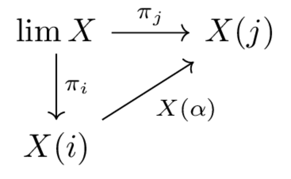
commutes, and so that, given another set of data (p, f_i: p to X(i)) with the same property, there is a unique map f: p \to \lim X so that f_i = \pi _if.
(I am sort of assuming you already know about limits, and just writing the definition above for convenience).
The proof idea, very weakly formulated, is that the adjunction lets us control maps into F(b), and the universal property of the limit is precisely about maps into F(\lim X).
Let's first make completely precise the claim: it is that, supposing (\lim X, \pi _i) forms a limit of X, then also (F(\lim X), F(\pi _i)) forms a limit of F \circ X. Note that this makes sense - F(\pi _i) really is a map from F(\lim X) to FX(i).
Now let's fix another cone (p,f_i) on (F\lim X, F(\pi _i)). We are attempting to construct a map p \to F(\lim X). This is equivalent to a map G(p) \to \lim X. We're going to construct _that_ map by constructing maps G(p) \to X_i. Where do we get those maps? We apply the adjunction again - they are simply the mates of the maps p \to F(X_i) we started with. Now we need to confirm that the map p \to F(\lim X) actually does make the desired triangles commute.
This follows from naturality of the adjunction, using the same property for G(p) \to \lim X: Consider the composite p \to F(\lim X) \to F(X(i)). By naturality of the adjunction (with regard to postcomposition), the mate of this map is the composite G(p) \to \lim X \to X(i). By construction, this equals the input map G(p) \to X(i), which is the mate of the original f_i: p \to F(X_i). Hence the composite has the same mate as f_i, so equals it.
The second thing we need to prove is that this map is unique with this property. We can do this by noting that, given two distinct map with this property, their mates G(p) \to \lim X are distinct (because the correspondence is bijective), and both have this property (by the same argument used above). This establishes the claim.
The homotopy theory of groups [the-homotopy-theory-of-groups]
- October 11, 2020
-
Eigil Fjeldgren Rischel
The homotopy theory of groups [the-homotopy-theory-of-groups]
- October 11, 2020
- Eigil Fjeldgren Rischel
Context: Krause and Nikolaus: Group Theory for Homotopy Theorists (pdf). Krause and Nikolaus develop group theory using model categories (well, one model category). This is obviously a joke, but I think it _is_ a very useful pedagogical joke. So I'm going to go through it and try to explain what's happening.
Group presentations
- October 11, 2020
-
Eigil Fjeldgren Rischel
Group presentations
- October 11, 2020
- Eigil Fjeldgren Rischel
If you've taken a course on group theory, you've probably learned about _presentations_ of a group. Here are some examples:
- \langle s,r | r^4, s^2 srsr \rangle - \langle a, b | \rangle - \langle a, b | aba^{-1}b^{-1} \rangle .
On the left of the pipe, we have a set S of _generators_. On the right of the pipe, we have a different set R of _relations_ - these are "group words" in the generators, i.e words involving both the generators and their inverses. The meaning of such a "presentation" is that it describes a group, namely the quotient of the free group on S by the relations.
Every group G has a presentation (in fact, many), for example given by taking S = G and R given by all words which evaluate to 1 in G. This leads to the idea that one could _define_ group theory out of presentations. This seems to work out well - in fact, given G,H groups, if we take their "canonical" presentations as above, a group homomorphism G \to H is exactly the same thing as a function G \to H which takes those words in G which evaluate to 1 to words in H which evaluate to 1.
However, this doesn't work in general - most group presentations don't have "enough generators" to represent all group homomorphisms into the presented group. And there are many maps which "should" be group isomorphisms which don't have an inverse on the level of presentations.
Model categories
- October 11, 2020
-
Eigil Fjeldgren Rischel
Model categories
- October 11, 2020
- Eigil Fjeldgren Rischel
The basic things you can do in a model category are:
- Invert certain maps that "should" be isomorphisms (or "equivalences") - Replace an object with a "better behaved" one which is "equivalent" in that sense.
Let's take a more classical example from "real" homotopy theory: Simplicial sets. In this context, we think of a simplicial set X as a "model" for a topological space, its geometric realization |X|. A map X \to Y is a simplicial homotopy equivalence if the map of spaces |X| \to |Y| is a homotopy equivalence of spaces. However, in many cases, such an equivalence can't be inverted, even up to (simplicial) homotopy. Similarly, there are often maps between geometric realizations which can't be represented by maps between the simplicial sets, even up to homotopy.
The basic solution to this is to work with certain nice simplicial sets called _Kan complexes_. A Kan complex has "enough simplexes" so that all the maps between them that "should" exist, do. Now we _could_ simply work with the category of Kan complexes - but this is an inconvenient category. Its main deficiency is probably that it does not have all colimits. This is compared to the full category of simplicial sets, which is as nice as they come.
So we use a powerful piece of technology called a _model structure_, making simplicial sets into a model category. (This is usually called the Kan model structure, or the Kan-Quillen model structure).
The upshot of this is that every simplicial set is homotopy equivalent to a Kan complex, in a very structured way which lets you use the technically convenient structure of the whole category of simplicial sets to describe "the homotopy theory of Kan complexes".
Back to groups
- October 11, 2020
-
Eigil Fjeldgren Rischel
Back to groups
- October 11, 2020
- Eigil Fjeldgren Rischel
Now we are going to try to adapt the above to groups.
The way to do this is to describe the _trivial cofibrations_ - essentially, these will be those maps which are "morally group isomorphisms".
Using the machinery of model categories, we can get away with specifying only a small "generating family". These are on page 2 of the paper.
Now here's a fun fact: this small list pins down exactly the "proper" presentations of groups, in this sense:
**Theorem**: The following two are equivalent for a presentation \langle S \mid R \rangle
- The map S \to F(S)/R is bijective, and R contains every word which is zero in F(S)/R. - For every diagram
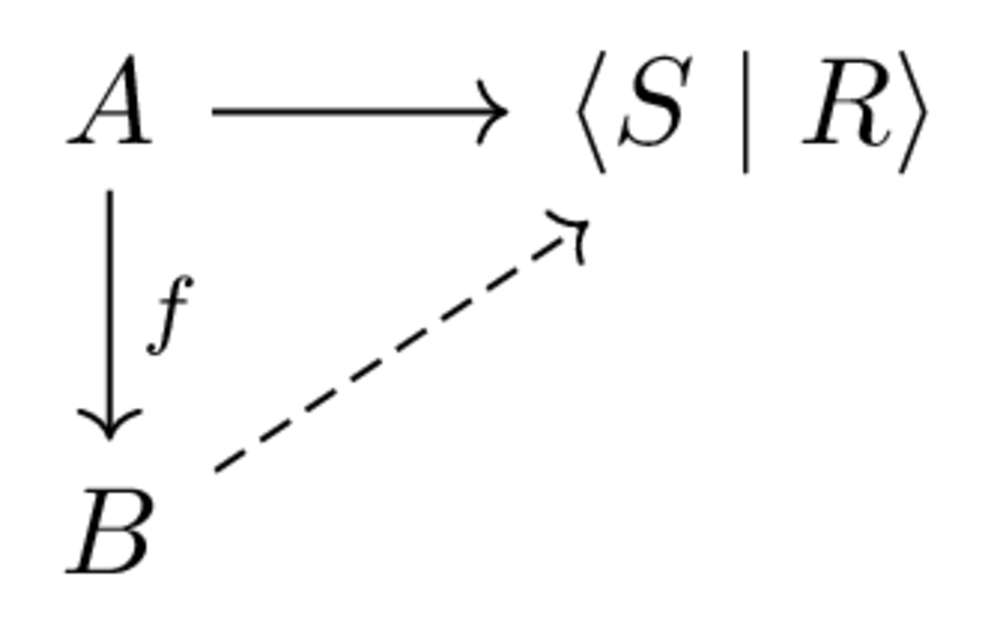
if f is in the generating list, there exists an extension like the dashed arrow making the triangle commute.
**Proof**: First, it's easy to check for each type of generating arrow that this holds:
- a and b must be sent to the same element (by injectivity), so we can simply send c there as well. - We can extend the map by sending a to whatever element w^{-1} evaluates to. - The remaining three maps simply add relations which are derivable from the existing ones - hence their images must already be in R.
Now for the other direction, suppose a,b \in S go to the same element in F(S)/R. Then the map \langle a,b \mid ab^{-1} \rangle \to \langle S \mid R \rangle does not have an extension over the first generating map. Hence that map is injective. Suppose w \in F(S)/R is not in S. Then the map \langle S \mid \emptyset \rangle \to \langle S \mid R \rangle does not extend over \langle S \sqcup \{a\} \mid a w^{-1} \rangle - there is nowhere to send a (since it must be sent to something that goes to w, for the property to hold). The statement that R contains every word that goes to zero means that R is stable under certain operations, which can similarly be proved from the morphisms.
It follows from the general theory of model categories that there always exists a map \langle S \mid R \rangle \to P into a "nice" (in technical terms, fibrant) presentation, which is itself a trivial cofibration. Understanding what the trivial cofibrations are in technical terms is more complicated - an argument going in the other direction from the one above will show that they are exactly those which correspond to group isomorphisms, but this might be a bit tricky.
A category of computable functions with runtime [category-of-computable-categories-with-runtime]
- October 9, 2020
-
Eigil Fjeldgren Rischel
A category of computable functions with runtime [category-of-computable-categories-with-runtime]
- October 9, 2020
- Eigil Fjeldgren Rischel
See: Giorgios Bakirtzis and Christian Williams: Turing Categories. Turing Categories describe _computability_. I want to find a category to work with _complexity_ instead. This is a stab at it. Fix a universal Turing machine and an encoding of the natural numbers. Of course, this lets us speak of _computable_ functions \mathbb {N} \to \mathbb {N} (and these don't depend on the choice of Turing machine). But fixing a specific machine also lets us speak of the _runtime_, in steps, of a program p with input n \in \mathbb {N}. Write p(n) = m if p(n) eventually terminates with output m, and write T(p,n) = t if it takes t steps.
Now we want to define a category as follows:
- The objects are subsets of the natural numbers.
- The maps A \to B are equivalence classes of programs under an "asymptotic equivalence" relation.
- The composition is "the obvious thing".
What I mean by asymptotic equivalence is this: the two programs halt on the same inputs, produce the same outputs, and run in the same amount of time up to a constant factor. To be more precise, p \lesssim p' : A \to B if there exists a constant C so that, when p(n) = m and T(p,n) = t, p'(n) = m and T(p,n) \leq Ct. Then p \sim p' if p \lesssim p' and p' \lesssim p.
This corresponds to our natural definition of "same behaviour, and same O-class".
Now, we want to construct the composition pp' simply to have pp'(n) = p(p'(n)) and T(pp',n) = T(p',n) + T(p,p'(n)). (This means that if p'(n) halts with output m, and p(m) halts with output k, then pp'(n) halts with output k, and has the runtime described above, otherwise it doesn't halt). It's not completely trivial that this is possible - essentially, the "overhead of composition" must be smaller than the runtime of the larger of p and p'. We must add this as a requirement to our Turing machine - luckily, this seems to be satisfied by most sane models of computation.
Call the category so defined \mathrm {Comp}.
Comp as a restriction category
- October 9, 2020
-
Eigil Fjeldgren Rischel
Comp as a restriction category
- October 9, 2020
- Eigil Fjeldgren Rischel
Given a program p: A \to B, we can define \bar {p}: A \to A as follows: to compute \bar {p}(n), run p(n) until completion, then return n no matter what.
Certainly any universal Turing machine admits this construction. Does this define a restriction category? Recall the axioms of a restriction category:
1. f\bar {f} = f 2. \bar {f}\bar {g} = \bar {g}\bar {f} 3. \overline {g\bar {f}} = \bar {g}\bar {f} 4. \bar {g}f = f\overline {gf}
(If these compositions are well-defined).
1. Clearly f\bar {f} has the same values as f. It runs in almost exactly twice the runtime of f, plus whatever the overhead of composition and the \bar {(-)} construction is. It is not actually completely obvious that this is small enough for _every_ universal Turing machine. Nevertheless, the assumption that T(\bar {p},n) \leq T(p,n) + C for some constant C seems rather harmless, which suffices here. 2. \bar {f}\bar {g} and \bar {g}\bar {f}, again, clearly have the same values. With the assumption from above, the runtime is also asymptotically the same. 3. Once again it's easy to see that the two maps have the same values. The first one runs in T(g,n) + T(f,n) + 2C, and so does the second one, hence they have the same (asymptotically) runtime. 4. Here the claim about equivalent runtimes is a bit more subtle. The first one takes T(f,n) + T(g,f(n)) time (up to asymptotic equivalence). The second one takes T(f,n) + T(g,f(n)) + T(f,n). But these two are equivalent - the second is at most twice the first.
Hence \mathsf {Comp} is a restriction category.
Comp as a Cartesian restriction category.
- October 9, 2020
-
Eigil Fjeldgren Rischel
Comp as a Cartesian restriction category.
- October 9, 2020
- Eigil Fjeldgren Rischel
Do "restriction products" exist in \mathsf {Comp}. This would seem to rely on a _constant-time_ bijection \mathbb {N} \cong \mathbb {N} \times \mathbb {N}. I am fairly sure this doesn't exist - since the encoding size of a natural number grows as the logarithm, it would seem that such a bijection must have unbounded runtime.
This may be remedied by passing to a less restrictive form of equivalence. For example, suppose we can find a logarithmic-time implementation of the above bijection. Then we can alter the definition of \lesssim so that p \lesssim p' as long as there exists C so that T(p',n) \leq CT(p,n)\log (n) (and they have the same values). There are other reasons to prefer this equivalence relation. It is not in general true that universal Turing machines can simulate each other with _constant_ overhead. This means that the choice of UTM made at the beginning of this post is actually significant. But it _is_ true that they can simulate each other with _logarithmic_ overhead. [^fn:1] This means the choice of machine is unimportant, making for a much nicer theory.
The construction of this correspondence does seem to be the only obstruction to equipping \mathsf {Comp} with a Cartesian restriction structure, in the "obvious" way (where A \times B is the subset of \mathbb {N} which corresponds under this bijection to a pair (a\in A, b \in B).)
Comp as a traced category
- October 9, 2020
-
Eigil Fjeldgren Rischel
Comp as a traced category
- October 9, 2020
- Eigil Fjeldgren Rischel
Can we define a trace operation on \mathsf {Comp}? This would be an operation Tr^X_{A,B}: Hom(A \times X \to B \times X) \to Hom(A,B). The idea would be that to evaluate Tr^X_{A,B}(f) on a \in A, you run f(a,0) to obtain b_1, x_1, then run f(a,x_1) to obtain b_2,x_2 and you keep doing this until you find a fixpoint where x_n = x_{n+1} then the resulting b_{n+1} is your output. (If this never terminates, you simply don't halt on that input).
The obvious problem is that the choice of 0 is non-canonical. We might want to let Tr^X_{A,B} only be defined when this input doesn't matter - but this property is not obviously computable! (We would have to check every possible n). This probably precludes Tr^X_{A,B} from satisfying the axioms of a trace. I'm not sure, but I think the issue will appear in the axiom Tr^X_{A,B}Tr^Y_{A\otimes X, B \otimes X}(f) = Tr^{X\otimes Y}_{A,B}(f). The right-hand side corresponds to applying f(a,0,0), then f(a,x_1,y_1), then proceeding like that until we find a fixpoint (x_n,y_n). In the second, we first define a function f(a,x) by applying f(a,x,0) to find y_1, then going until we find a fixpoint y_n. Then we apply _the function to defined_, call it f', with f'(a,0) to find x_1, and so on. In other words, we first find a fixpoint y for f(a,0,y), and use that fixpoint to produce x_1. Then we find a fixpoint for f(a,x_1,y) and so produce y_2, and so on. This does eventually produce a pair (x,y) which form a fixpoint for f(a,x,y), but not necessarily the same one as the "simultaneous" procedure. This problem is exactly fixed if we only allow those as where the starting input doesn't matter - then there is a unique fixpoint, and we are happy.
The second problem, of course, is that the two procedures defined above have _very different runtimes_. This problem does seem to be baked into the axioms of a traced monoidal category. This is perhaps not surprising - these axioms are not saying that both sides are equally fast ways of computing the result, just that the results are equal. So perhaps we should look for some alternative "complexity-sensitive" version of these axioms that make sense in our context.
On the other hand, the temptation to regard a string diagram with loops as describing a meaningful program is very strong. This would suggest that we need a different version of \mathsf {Comp}, or perhaps a different traced structure, that makes the two sides of the equation equal.
Comp as a Turing category
- October 9, 2020
-
Eigil Fjeldgren Rischel
Comp as a Turing category
- October 9, 2020
- Eigil Fjeldgren Rischel
Comp is, first of all, not a Turing category, because undecidable subsets of the natural numbers won't be retracts of them. If we fiddle with the definition to fix this issue (we can remove all other objects than \mathbb {N} and \{1\}, for example), it might actually be a Turing category - because of the fact that universal Turing machines can simulate each other with logarithmic overhead.
Further questions
- October 9, 2020
-
Eigil Fjeldgren Rischel
Further questions
- October 9, 2020
- Eigil Fjeldgren Rischel
- What is the general definition of which \mathsf {Comp} is an example? - Does this actually help at all? - Is there a (family of) model(s) of computation which allows us to A: make a category with useful internal structure, B: without fiddling with various notions of asymptotic performance.
[^fn:1]: See eg Wikipedia
Localizations of categories of dynamical systems [localizations-categories-dynamical-systems]
- October 4, 2020
-
Eigil Fjeldgren Rischel
Localizations of categories of dynamical systems [localizations-categories-dynamical-systems]
- October 4, 2020
- Eigil Fjeldgren Rischel
See also: Jade Master: Dynamical Systems With Category Theory? Yes!, This tweet by me.
Discrete dynamical systems
- October 4, 2020
-
Eigil Fjeldgren Rischel
Discrete dynamical systems
- October 4, 2020
- Eigil Fjeldgren Rischel
A discrete dynamical system (S,T) consists of a set S and a time-step function T: S \to S. It's clear that this is exactly the same thing as a \mathbb {N}-set, i.e a set with an action of the monoid (\mathbb {N},+,0)[^fn:1]. A "morphism of discrete dynamical systems" is just the obvious thing, namely a map which preserves the action - an equivariant map.
For now, we will restrict ourselves to those dynamical systems with "time-reversible dynamics" - that is, those where the action T: S \to S is a bijection. The subcategory of such things inside \mathbb {N}-\mathsf {Set} is equivalent to \mathbb {Z}-\mathsf {Set} - a dynamical system is time-reversible if and only if the action of \mathbb {N} extends to an action of \mathbb {Z}.
Now, we will be interested in _localizations_ of the category \mathbb {Z}-\mathsf {Set}. One important family of such localizations comes from the group homomorphisms \mathbb {Z} \to \mathbb {Z}/n.
This homomorphism gives a functor \mathbb {Z}/n-\mathsf {Set} \hookrightarrow \mathbb {Z}-\mathsf {Set}. In fact, this functor is fully faithful, and its image is exactly the subcategory of n-periodic dynamical systems - i.e those for which T^n(x) = x for all x \in S. Moreover, this functor admits a left adjoint L_n. It takes a dynamical system (S,T) to (S/\sim , \bar {T}), where \sim is the equivalence relation generated by x \sim T^nx and \bar {T} is the induced map.
The order structure of this family of localizations is exactly the division order. By which I simply mean, if n | m, then an n-periodic dynamical system is also m-periodic, and if every n-periodic dynamical system is m-periodic, then n|m (proof of the second implication: consider the dynamical systen (\mathbb {Z}/m, +1)).
Using these, we can form a sort of "p-adic completion" of any dynamical system, as the limit \lim _n L_{p^n} S =: S^{\wedge }_p. The functor (-)^\wedge _p is a localization. The p-adic completion of the integers with translation action is exactly the p-adic integers (with translation action). Since each system S/p^n acquires a canonical action of \mathbb {Z}/p, it would seem that probably S^\wedge _p acquires an action of the p-adics \mathbb {Z}^\wedge _p.
However, to make sense of this, it's probably best to work in a category of topological spaces with continuous group actions. I would guess that the \mathbb {Z}/p actions assemble to a unique _continuous_ \mathbb {Z}_p^\wedge action, although I have not checked it.
The family of localizations (-)^\wedge _p is jointly conservative on _finite_ dynamical systems (since each orbit is an n-period for some n). However this fails in a predictable way in the infinite case, where we can't distinguish between (\mathbb {Z},+) and (\hat {\mathbb {Z}},+). To remedy this, one would need some sort of "rationalization" of dynamical systems. However, there we run into the issue that the functor \mathbb {Q}-\mathsf {Set} \to \mathbb {Z}\mathsf {Set} is not fully faithful - a \mathbb {Q} set has a chosen "half action", the action of 1/2 on S, but this action is not necessarily uniquely determined by the action of 1.
Smooth dynamical systems
- October 4, 2020
-
Eigil Fjeldgren Rischel
Smooth dynamical systems
- October 4, 2020
- Eigil Fjeldgren Rischel
We take a somewhat unorthodox approach and let a _smooth dynamical system_ be a smooth manifold M with an action of the Lie group \mathbb {R}. (Again, we are looking at time-reversible systems). Given a discrete subgroup of \mathbb {R}, the quotient \mathbb {R}/H is again a Lie group, and we obtain a fully faithful inclusion \mathbb {R}/H-\mathsf {Mdf} \hookrightarrow \mathbb {R}-\mathsf {Mdf}.
The discrete subgroups of \mathbb {R} all have the form \lambda \mathbb {Z} for some \lambda , and the quotient is always diffeomorphic to S^1. As above, passing to this quotient corresponds to considering λ-periodic systems.
In this situation, there no longer exists a left adjoint, for annoying reasons. The universal property of the left adjoint, if written out, tells us it should take a manifold M to the quotient M/(\lambda \mathbb {Z}) of the action by \lambda \mathbb {Z}. Consider the normal additive action of \mathbb {R} on S^1 = \mathbb {R}/\mathbb {Z}. If we take \lambda to be an irrational number, the orbits of the action are dense in S^1, and the quotient is not even a topological manifold.
One would hope this problem can be solved by something like "derived manifolds", but I haven't looked into that yet.
[^fn:1]: My natural numbers include 0
Cheap nonstandard analysis [cheap-nonstandard-analysis]
- October 2, 2020
-
Eigil Fjeldgren Rischel
Cheap nonstandard analysis [cheap-nonstandard-analysis]
- October 2, 2020
- Eigil Fjeldgren Rischel
Terry Tao: A cheap version of nonstandard analysis. MathOverflow: Does Cheap Nonstandard analysis take place in a topos? (Answer: Yes, but an elementary topos, not a Grothendieck topos).
This is partially a summary of Tao's blog post, partially a small discussion of way LEM fails for cheap nonstandard reals.
What is "nonstandard analysis"?
- October 2, 2020
-
Eigil Fjeldgren Rischel
What is "nonstandard analysis"?
- October 2, 2020
- Eigil Fjeldgren Rischel
In "normal" nonstandard analysis, we consruct the "nonstandard reals" \mathbb {R}^* as an ultrapowwer of the ordinary reals with regards to some nonprincipial ultrafilter \mathfrak {u}. This means that a nonstandard real is a sequence (x_n) of reals, quotiented by the equivalence relation which identifies two sequences if the set of naturals where they agree is in the ultrafilter - in symbols, \{n | x_n = y_n\} \in \mathfrak {u}
This set inherits all the structure of the reals - where addition and multiplication is pointwise, and (x_n) \leq (y_n) if \{n | x_n \leq y_n\} \in \mathfrak {u}. In fact, it is even a totally ordered field, since first-order properties pass to ultrapowers by Łoś's Theorem. It also contains a copy of the real numbers, where x \in \mathbb {R} is identified with a constant sequence. We call these the _standard reals_.
(\mathbb {R}^* is not complete, since this is a second-order property.)
\mathbb {R} contains "infinitesimals", like the sequence (1/n) - this is a positive nonstandard real number, but less than every positive standard real number. Call this number \epsilon .
It also contains "infinite numbers", like the sequence (n) - this is a nonstandard real wich is larger than every standard real.
Given a function f: \mathbb {R}^* \to \mathbb {R}^*, we can ask for the value \frac {f(x + \epsilon ) - f(x)}{\epsilon }. This is a well-defined nonstandard real, since \epsilon is not zero. In fact, it is the nonstandard real \left (\frac {f(x + 1/n) - f(x)}{1/n}\right ). If f comes from a function \mathbb {R} \to \mathbb {R} which is differentiable, this sequence converges to f'(x). This means that the difference between the nonstandard derivative and the normal derivative is an infinitesimal, in the sense that it is smaller than every positive and larger than every negative standard real. One can show that f'(x) is the only standard real with this property - so this gives a definition of the derivative (which does not depend on the choice of \epsilon ).
Nonstandard analysis takes this idea and runs with it to develop various parts of analysis using these infinitesimals.
Cheap nonstandard analysis
- October 2, 2020
-
Eigil Fjeldgren Rischel
Cheap nonstandard analysis
- October 2, 2020
- Eigil Fjeldgren Rischel
There are a few problems with this:
- The existence of a non-principal ultrafilter on \mathbb {N} requires some "unfortunate" axiom like the axiom of choice or somesuch. (The existence of non-principal ultrafilters on all infinite sets is called the ultrafilter theorem, and is strictly weaker than the axiom of choice, but still considered a bit suspicious - for instance it implies the existence of nonmeasurable sets). - According to Tao, it's sometimes difficult to extract a quantitative bound from an asymptotic theorem proved with nonstandard analysis - he links this to the first point.
However, these difficulties disappear if we instead use the Frechet filter, consisting of all cofinite sets, on \mathbb {N}. In other words, a cheap nonstandard real is a sequence (x_n) of reals, quotiented by the equivalence relation that (x_n) = (y_n) if x_n = y_n for n sufficiently big. Note that the Frechet filter is not an ultrafilter! Hence Łós' theorem does not hold, so the cheap nonstandard reals fail to inherit all the good properties of the ordinary reals.
The easiest example of this is that they are not a field. To see this, consider the cheap nonstandard real (0,1,0,1,0,1,\dots ). This is not equal to zero, because there are infinitely many ones. On the other hand, it is also not invertible: if we multiply it with the cheap nonstandard real (x_n), we get (x_1, 0, x_2, 0, \dots ). This is not equal to one, because there are infinitely many zeroes.
The way this would work for an ultrafilter is that either the set of even numbers or odd numbers would be in the ultrafilter. So either (0,1,0,1,\dots ) is zero or one - in either case, it's clearly invertible.
It turns out the parts of Łós' theorem that specifically fails for non-ultra filters are about statements \phi \vee \psi - disjunction, and \neg \phi - negation. Hence the statement x = 0 \vee (\exists y : xy=1) doesn't hold for the quotiented product, even though it holds for the ultraproduct.
However, this shouldn't concern us _too much_, because we can basically view this as a faily of LEM (in a way that I will explain), and LEM is another one of those slightly suspicious axioms.
In what sense does LEM fail for cheap nonstandard reals? As mentioned, the nonstandard reals are a model of the language of ordered fields. The way this works is that any formula \phi (x) in that language can be interpreted for a nonstandard real by asking if \phi (x_n) holds for a set in the ultrafilter - for short, whether \{n \mid \phi (x_n)\} \in \mathfrak {u}. A priori, this gives two ways of intepreting a formula like x=0 \vee x=1. We can ask whether \{n \mid x_n = 0 \vee x_n = 1\} \in \mathfrak {u}, or we can ask whether \{n \mid x_n = 0\} \in \mathfrak {u} \vee \{n \mid x_n=0\} \in \mathfrak {u}. The second is the "correct" semantics for first-order logic, but the first is usually more convenient. Luckily, for ultrafilters they are the same.
We can try to use this approach with a non-ultrafilter, like the Frechet filter \mathcal {F}. But now there's a difference! If we let (x_n) = (0,1,0,1,\dots ), it's true that \{n \mid x_n = 0 \vee x_n = 1\} \in \mathcal {F}, but not true that \{n \mid x_n = 0\} \in \mathcal {F} \vee \{n \mid x_n = 1\} \in \mathcal {F}. A similar problem crops up for negation.
In this way, LEM fails in some sense, because we can have \phi ,x so that \{n \mid \phi (x_n)\} \notin \mathcal {F} and \{n \mid \neg \phi (x_n)\} \notin \mathcal {F}.
Do observe however that here the "or" is being interpreted _externally_, but the "not" is being interpreted _internally_.
Jensen-Shannon divergence is compositional [jsd-as-enrichment]
- June 12, 2020
-
Eigil Fjeldgren Rischel
Jensen-Shannon divergence is compositional [jsd-as-enrichment]
- June 12, 2020
- Eigil Fjeldgren Rischel
Let \mathsf {FinStoch} be the category of finite sets and stochastic matrices. Given two stochastic matrices, f_1,f_2: X \to Y, we can define their **Jensen-Shannon distance** as d(f_1,f_2) := \sup _x \sqrt {\operatorname {JSD}(f_1(x),f_2(x))}, where JSD is the Jensen-Shannon divergence. It's a standard result that the root of JSD defines a metric on the space of probability measures - hence the above defines a metric on the set \mathsf {FinStoch}(X,Y). My aim here is to show that _this gives an enrichment of \mathsf {FinStoch} in the category \mathsf {Met} of metric spaces and **short**, i.e distance nonincreasing, maps_
The content of this statement is that the composition map
\mathsf {FinStoch}(X,Y) \otimes \mathsf {FinStoch}(Y,Z) \to \mathsf {FinStoch}(X,Z) is a short map. The monoidal structure on \mathsf {Met} that we're considering is given by the "1-metric", i.e
d_{X \otimes Y}((x,y),(x',y')) = d_X(x,x') + d_Y(y,y')This has the convenient property that a map is short if and only if it's "short in each variable separately". In other words, we must show that the map
f \circ - :\mathsf {FinStoch}(X,Y) \to \mathsf {FinStoch}(X,Z)is short for each f, and that the map
- \circ f : \mathsf {FinStoch}(Y,Z) \to \mathsf {FinStoch}(X,Z)is short for each f.
Fact about \operatorname {JSD}.
- June 12, 2020
-
Eigil Fjeldgren Rischel
Fact about \operatorname {JSD}.
- June 12, 2020
- Eigil Fjeldgren Rischel
We will use the following characterization of \operatorname {JSD}(p,q): Let B be a "fair coinflip", i.e a random variable which is 0 with probability 1/2 and 1 otherwise. Let X be a random variable which is distributed according to p if B=0 and q if B=1. Then the mutual information of X and B is exactly the Jensen-Shannon divergence of p and q
Postcomposition
- June 12, 2020
-
Eigil Fjeldgren Rischel
Postcomposition
- June 12, 2020
- Eigil Fjeldgren Rischel
We want to show that d(fg_0,fg_1) \leq d(g_0,g_1). Clearly we may as well square both sides, so that we're trying to show that
\sup _x \operatorname {JSD}(fg_0(x),fg_1(x)) \leq \sup _x \operatorname {JSD}(g_0(x),g_1(x))It suffices to show that this inequality holds for each x, so let an x be given. Then \operatorname {JSD}(g_0(x),g_1(x)) is the mutual information between a fair coin B and a variable Y distributed according to g_B(x). and \operatorname {JSD}(fg_1(x),fg_2(x)) is the mutual information between B and a variable distributed as f(Y). But "postprocessing" by f can't possible put more information about B into the random variable, since it depends on Z only through B. Hence we have the desired inequality.
Precomposition
- June 12, 2020
-
Eigil Fjeldgren Rischel
Precomposition
- June 12, 2020
- Eigil Fjeldgren Rischel
We want to show d(g_0f,g_1f) \leq d(g_0,g_1) Again it suffices to show
\sup _x \operatorname {JSD}(g_0f(x),g_1f(x)) \leq \sup _y \operatorname {JSD}(g_0(y),g_1(y))It's enough to show this for each specific x, so let's assume wlog that X=\ast and f is simply a distribution, and we're showing
\operatorname {JSD}(g_0f,g_1f) \leq \sup _y \operatorname {JSD}(g_0(y),g_1(y))To see this, let Y be distributed according to f, let B be an unbiased coin, and let Z be distributed according to g_B(Y). Then \operatorname {JSD}(g_0f,g_1f) is I(Z;B), and \operatorname {JSD}(g_0(y),g_1(y)) is I(Z;B | Y = y).
Our claim is that I(Z;B) \leq I(Z;B | Y=y) for at least one y. We insert the entropy formula for mutual information:
H(B) - H(B|Z) \leq H(B|Y=y) - H(B|Z, Y=y)Since B,Y independent, H(B|Y=y) = H(B) (equals one bit), so we may rearrange this as H(B|Z,Y=y) \leq H(B|Z) Now that the expected value E_y[H(B|Z,Y=y)] is precisely H(B|Z,Y) by definition. By a standard inequality H(B|Z,Y) \leq H(B|Z). Hence we also have the inequality H(B|Z,Y=y) for at least one y, as desired.
Followup questions
- June 12, 2020
-
Eigil Fjeldgren Rischel
Followup questions
- June 12, 2020
- Eigil Fjeldgren Rischel
1. Is there a way to build something like this "canonically" - the way entropy is characterized by a set of axioms in A characterization of Entropy in Terms of Information Loss? 2. How does this relate to other metrics on probability, i.e the description from A probability monad as the colimit of spaces of finite samples
Compositionality for Transfer Learning [compositionality-for-transfer-learning]
- June 2, 2020
-
Eigil Fjeldgren Rischel
Compositionality for Transfer Learning [compositionality-for-transfer-learning]
- June 2, 2020
- Eigil Fjeldgren Rischel
_Transfer learning_ is the idea that, after a machine learning system (or a non-machine learning system, for that matter, like a human) has learned to solve some problem, it should be able to _transfer_ this knowledge to solving similar problems. Humans are pretty good at this, at least compared to current ML systems, which tend to suck.
Why do we expect transfer learning to work? It seems that, in general, we expect that the solution to a task can be _decomposed_ into several pieces, some of which will still be useful for the related task. As an example, suppose we teach a self-driving card to drive to a given place, using a map of the local area and camera input. If we could open up the resulting algorithm, we may expect to find "subroutines" corresponding to
1. Breaking down the visual input into objects. 2. Maintaining/updating an internal memory with this data. 3. Using this data to locate itself on the map 4. Plotting a route on the map between two points 5. Executing a route while driving correctly (i.e not breaking the law, not causing crashes).
If we now want this system, instead, to locate and follow a car with a specific license plate (or something), we would expect that most of these routines, except perhaps 3 and 4, would still be useful. It would not have to learn all over again how to recognize other cars and involve crashes.
In other words, we expect transfer learning to happen because of _compositionality_. To introduce some symbols, we are trying to learn a function f: X \to Y from observations to decisions. The target behavior is really a function of some high-level description of the system, as understood by humans, i.e it factors as X \overset {p}{\to } \bar {X} \overset {f'}{\to } Y. If the system manages to learn p as well as f', then if we swap out the task with another one, which is also specified on the same abstract level, g': \bar {X} \to Y, the system will have less to do - a lot of the parameter space is already in the right configuration.
Of course, if you already knew how to compute the high-level representation \bar {X}, you mostly wouldn't need machine learning. However, when we view the problem from this angle, it seems one way to get more transfer learning is to look for learning algorithms that output "decomposed" models, so that we can try to separate the abstraction X \to \bar {X}, from the "task-specific logic" f': \bar {X} \to Y.
One way to do this is to find a class of related tasks, \{f_i:X \to Y_i | i = 1 \dots n\}, which we feel share a common abstraction. Then we can pick some set \bar {X} and try to train n+1 models - one going from X \to \bar {X}, the others going from \bar {X} \to Y_i. We give each of these algorithms the average loss across all the tasks as the loss. Then the "high-level models" \bar {X} \to Y_i try to make use of the low-level data as best they can, while the "abstraction" model X \to \bar {X} tries to create an abstraction which is useful to all the high-level models.
Stochastic Stalks [stochastic-stalks]
- May 24, 2020
-
Eigil Fjeldgren Rischel
Stochastic Stalks [stochastic-stalks]
- May 24, 2020
- Eigil Fjeldgren Rischel
Stalks and points
- May 24, 2020
-
Eigil Fjeldgren Rischel
Stalks and points
- May 24, 2020
- Eigil Fjeldgren Rischel
Recall that a point of a topos \mathcal {E} is a geometric morphism from the topos Set. My preferred way to think about this is to consider the sheaf topos Sh(X) on some (sober) topological space X. Then given x \in X and a sheaf S, we can form the stalk at x
S_x := \operatorname {colim}_{x \in U \subseteq X \text { open}} S(U)
1. This determines the point uniquely, i.e if (-)_x \simeq (-)_y then x = y 2. This is a left exact left adjoint Sh(X) \to Set - i.e part of a geometric morphism Set \to Sh(X). 3. All left exact left adjoints Sh(X) \to Set have this form.
Hence it makes sense to identify literal points of X with points of Sh(X) in the above sense.
Random points
- May 24, 2020
-
Eigil Fjeldgren Rischel
Random points
- May 24, 2020
- Eigil Fjeldgren Rischel
We can think of a probability measure on a space X as a sort of "generalized point", which has been "smeared out". How can we lift this intuition to the level of Sh(X)? It seems sort of obvious that we shouldn't expect this to work on the level of sets - they are somehow too "discrete" to capture quantitative information about probabilities. It's actually worth mentioning here that any point of Sh(X) is determined by its action on sheaves represented by open sets, which must each be sent to either \emptyset or * (this follows from the "left exact left adjoint" assumptions). The fact that it's a left exact left adjoint furthermore implies that it must be a sort of infinitely-additive \{0,1\}-valued probability measure defined on the open sets, and it follows from this that it's a "dirac measure". This is how to prove that all points are really represented by a point. It seems that one way of considering "random points" would be to let the functor take values in a category with objects that can reasonably represent more complicated probability measures. It also seems unlikely that we can rely completely on universal properties to carry the day here. If U, V \subset X are open sets, then U \cap V is their product, both in O(X) and in Sh(X). So if a functor P: Sh(X) \to C preserves products, P(U \cap V) depends only on P(U) and P(V) - so this clearly can't capture all possible probability measures.
One attempt: Stochastic stalks
- May 24, 2020
-
Eigil Fjeldgren Rischel
One attempt: Stochastic stalks
- May 24, 2020
- Eigil Fjeldgren Rischel
I haven't solved this problem completely (I'm not convinced a good general solution exists). One approach is to think about _integration of metric spaces over a measure_, which I will now explain. A _sheaf of metric spaces_ is a functor O(X)^{op} \to Met, where Met is the category of metric spaces and _short_, i.e distance-nonincreasing, maps, which satisfies the sheaf axiom. We denote the category of such sheaves by Sh(X,Met). By "the sheaf axiom", I mean it preserves limits. Since Met does not have all limits, this is a bit subtler than it may appear. However, since Met does have finite limits, this difficulty disappears if we assume X is compact.
Let M be a sheaf of metric spaces and let P be a Radon probability measure on X. Then we define M_X to be the product \prod _{x \in X}M_x of all the stalks (just considered as a set). Equip M_X with a pseudometric d by setting d(a,b) = \int d(a_x,b_x)P(dx). In other words, we _integrate_ the distances according to the given probability measure. If we quotient out with the relation a \sim b if d(a,b) = 0, this gives a proper metric space, M_X/\sim .
Now for each U \subset X with P(U) = 1, we consider the map M(U) \to M_X/\sim given by taking all the germs. We let M_P be the metric space consisting of the images of all these maps.
This defines a functor Sh(X,Met) \to Met. We can recover the probability measure on an open set A by considering a sheaf M given by two points at distance 1 if U \subset A and the singleton otherwise. Then M_P consists of two points at distance P(A). At least in the case of compact Hausdorff spaces, this determines the underlying measure uniquely. (In general, the "measure defined on open sets" that we recover in this way is called a valuation, and you can argue that we shouldn't expect to tell the difference between different measures with the same valuation).
Questions
- May 24, 2020
-
Eigil Fjeldgren Rischel
Questions
- May 24, 2020
- Eigil Fjeldgren Rischel
- What useful properties characterize functors of the above form? - Is there a good way of doing this for \sigma -algebras instead of topologies? - Is there a good way of doing this for a general topos?
Example: Random variables
- May 24, 2020
-
Eigil Fjeldgren Rischel
Example: Random variables
- May 24, 2020
- Eigil Fjeldgren Rischel
Let M be any metric space. Then we can form a sheaf of metric spaces where M(U) is the set of continuous functions U \to M in the sup metric. Then the metric space M_P is the set of M-valued random variables, metrized by letting d(A,B) := \mathbb {E}_P(d(A,B)) - i.e metrized by _expected_ distance.
The Ax-Grothendieck theorem [ax-grothendieck-model-theory]
- May 17, 2020
-
Eigil Fjeldgren Rischel
The Ax-Grothendieck theorem [ax-grothendieck-model-theory]
- May 17, 2020
- Eigil Fjeldgren Rischel
The Ax-Grothendieck theorem says the following: Let f: \mathbb {C}^n \to \mathbb {C}^n be a polynomial function. If it's injective, then it's surjective as well.
Here's how to prove it:
1. The statement can be formulated as a first-order statement in the language of fields 2. If a statement like that fails for \mathbb {C}, there's a disproof in the first-order theory of algebraically closed fields of characteristic zero. 3. Such a proof is _finite_, so it only uses finitely many of the assumptions p \neq 0 - hence the theorem also fails in algebraically closed fields of sufficiently high characteristic. 4. Hence it fails in the algebraic closure of \mathbb {F}_p. The specific counterexample is in some finite extension of \mathbb {F}_p, which is a finite field. But clearly the theorem is _true_ for finite fields, just by counting.
I think this is a pretty cool proof - it uses model theory in a really surprising way, and the step where you use the fact that _proofs are finite_ is just totally bonkers.
First-order logic and completeness
- May 17, 2020
-
Eigil Fjeldgren Rischel
First-order logic and completeness
- May 17, 2020
- Eigil Fjeldgren Rischel
Recall that first-order logic works with statements built up out of the logical connectives \wedge , \vee , \neg , \Rightarrow \bot , \top , \forall , \exists , =. The language of _fields_ augments these symbols with +, -, \cdot , 1, 0 (it's really just the language of commutative rings - being a field just means that additional axioms hold).
A statement in the first-order language of fields could be something like this:
\forall a,b: \neg (a = 0) \Rightarrow \exists x: a\cdot x + b = 0
This statement says that all nonconstant linear polynomials have a solution, which is true.
We could also write down a statement like \forall a, b, c, d, e: \neg (a = 0) \Rightarrow \exists x: a x^4 + bx^3 + cx^2 + dx + e = 0
This says that all fourth-order polynomials have a root, which is not always true, but true sometimes, like in \mathbb {C}.
Similarly, we can form a statement R_n for all n \in \mathbb {N}, saying that all nth order polynomials have a root. Note that the conjunction of all these statements is _not_ a first-order statement in itself - we can't take conjuctions of infinitely many statements, and there's no way to quantify over all polynomials in the theory of fields.
Similarly, we can form statements like 1+1 \neq 0. This is also true in \mathbb {C}, but fails in fields of characteristic 2. We can form statements C_n for all n, saying that n \neq 0 - that the field does not have characteristic n.
The _theory of algebraically closed fields of characteristic zero_ is the theory consisting of the axioms of a field augmented with the statements C_n and R_n for all n. A model of this theory is precisely an algebraically closed field of characteristic zero (hence the name).
Now here is a highly nontrivial fact about this theory: it is _complete_. This means that _any statement expressible in the first-order language of fields is either provable or disprovable in it_. This means that, from the perspective of first-order logic, there are really no differences between fields of this type - even though there are of course many different such fields, they have the same first-order properties.
Ax-Grothendieck in first order
- May 17, 2020
-
Eigil Fjeldgren Rischel
Ax-Grothendieck in first order
- May 17, 2020
- Eigil Fjeldgren Rischel
We want to phrase the Ax-Grothendieck theorem as a first-order statement. It turns out this isn't quite possible, because we can't quantify over "all degree d polynomials" or "all n \in \mathbb {N}". Therefore we instead formulate the statement P(n,d): "Any polynomial function f : \mathbb {C}^n \to \mathbb {C}^n of degree at most d is surjective if it's injective". Then the Ax-Grothendieck statement says that P(n,d) holds for all n \geq 1, d \geq 0 (By the way: by "polynomial \mathbb {C}^n \to \mathbb {C}^n", I mean a function where each coordinate is an n-variable polynomial)
How does P(n,d) look as a first-order formula? It's quite complicated - mostly because a degree d polynomial like f involves a large number of coefficients. The main point is that there is a _definite_ number of coefficients, once n and d is fixed, and so we can write "for all choices of coefficients for f..." in first-order logic. For instance, if d = 2, n=1, this looks like \forall a_{11},a_{12},a_{21},a_{22},b_1,b_2 \dots Here a_{12} is the coefficient for x_1 in the second coordinate polynomial of f, and so on.
Now of course we can also make sense of injectivity: it's just the statement f(x_1,\dots x_n) = f(x'_1, \dots x'_n) \Rightarrow x_1=x'_1 \wedge \dots \wedge x_n = x'_n - where the equality on the left of the implication is shorthand for a complicated expression involving the coefficients of f.
And we can make sense of surjectivity: it just means \forall y_1 \dots y_n, \exists x_1, \dots x_n: f(x_1, \dots x_n) = (y_1, \dots y_n) Hence we have all the ingredients to make sense of P(n,d).
Finishing up the proof
- May 17, 2020
-
Eigil Fjeldgren Rischel
Finishing up the proof
- May 17, 2020
- Eigil Fjeldgren Rischel
We now have most of the ingredients to fill out the proof above. Since Ax-grothendieck is a (family of) first-order statements, if it fails, there is a disproof in the first-order theory of algebraically closed characteristic zero fields. To be specific, if Ax-Grothendieck is false, then P(n,d) is false for some specific n,d, and hence there is a disproof of that statement, i.e a proof of \neg P(n,d).
Observe that such a proof is finite. Hence it can use at most finitely many of the statements C_n. Hence for p large enough (larger than any n where C_n is used in the proof), Ax-Grothendieck fails for algebraically closed fields of characteristic p - like the algebraic closure of \mathbb {F}_p. (How do we know it fails? We have a proof that it fails!) Hence there exists some polynomial function f: \overline {\mathbb {F}_p}^n \to \overline {\mathbb {F}_p}^n which is injective and not surjective. But now we can take the algebraic extension of F_p by all the coefficientsof f and the coordinates of a point y \in \overline {\mathbb {F}_p}^n which is not in the image. Call this extension L. Then f: L^n \to L^n is a well-defined injective polynomial which is not surjective. And since L is a finite extension of a finite field, it's finite. But then we clearly have a contradiction: injective fuctions between finite sets of the same cardinality are bijections, just by counting.
This concludes the proof.
Notes from "Persistent Homotopy Theory" [jardine-persistent-htpy]
- May 10, 2020
-
Eigil Fjeldgren Rischel
Notes from "Persistent Homotopy Theory" [jardine-persistent-htpy]
- May 10, 2020
- Eigil Fjeldgren Rischel
My notes from Persistent Homotopy Theory by JF Jardine. The goal of the paper is to study "filtered spaces". By this is meant in general something like an assignment s \mapsto X_s of a "space" or simplicial set to each nonnegative real s \in [ 0,\infty ). A prototypical example is the Vietoris-Rips complex of a metric space, V_s(X).
The idea being pointed towards is some sort of modification of model category theory to make ideas from persistent homology work more nicely. The main example considered is an inclusion of VR-complexes V_s(X) \to V_s(Y) coming from an incusion of datasets X \subset Y where all the points in Y are "close to" ponts in Y. In this situatio V_s(X) \to V_s(Y) is not generally a homotopy equivalence or anything like tat, but it's still a bit "equivalency" - we would like to understand howthis works, and how this plays into classical model category theory.
1 Posets
- May 10, 2020
-
Eigil Fjeldgren Rischel
1 Posets
- May 10, 2020
- Eigil Fjeldgren Rischel
Given a finite subset X of a metric space Z, which we think of as a _data set_, we consider the collection P_s(X) of subsets \sigma \subset X where d(x,y) \leq s for all x,y \in \sigma . We can order this by inclusion - it is exactly the poset of simplices in the Vietoris-Rips Complex V_s(X).
Now we want to work with this combinatorial data as if it were topological data. This is generally easiest if we're working with a simplicial set. We can make this into a simplicial set by choosing an ordering on X, but this is non-canonical. We can also consider the nerve B(P_s(X)), but this is somewhat clunky - the resulting simplicial structure is really the _subdivision_ of the complex V_s(X). (B for the nerve of a category - a simplicial set - it somewhat unusual notation, but I've stuck with Jardine's choice of notation.)
2 Stability
- May 10, 2020
-
Eigil Fjeldgren Rischel
2 Stability
- May 10, 2020
- Eigil Fjeldgren Rischel
Define the Hausdorff Distance on finite subsets X,Y \subset Z of a metric space as follows: d_H(X,Y) < r if and only if for all x there exists y with d(x,y) < r, and vice versa.
Then a situation of interest is if we have two data sets with "small" Hausdorff distance - in this case, the datasets seem to reflect mostly the same underlying topology, so we'd like our methods to give mostly the same results.
What sort of relation do we have between P_s(X) and P_s(Y)? For simplicity let's work with the case where X \subset Y. Then we have an inclusion i: P_s(X) \to P_s(Y), and we can ask in what sense this is "equivalence-like". We can try to cook up an inverse by picking a nearest point \theta (y) \in X for each y \in Y. By assumption d(y,\theta (y)) < r. This means we can build a diagram
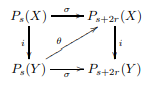
The top square commutes - in other words, i almost has a retract, except we have to add an extra error of up to 2r. The bottom square doesn't commute - after all, \theta does really move around some points. But it doesn't move around points too much - the set \sigma (t) \cup i(\theta (t)) is still in P_{s+2r}(Y), i.e: the altered points and the original points are all within 2r of each other. The pair of inclusions \sigma (t) \hookrightarrow \sigma (t) \cup i(\theta (t)) \hookleftarrow i(\theta (t)) present a _homotopy_ between i\theta and \sigma , so the bottom square commutes up to homotopy. In other words, i and \theta form a sort of "approximate deformation retract".
3 Controlled equivalences
- May 10, 2020
-
Eigil Fjeldgren Rischel
3 Controlled equivalences
- May 10, 2020
- Eigil Fjeldgren Rischel
In this section we encounter some interesting homotopy theory-ish things. We consider the category of functors [ 0,\infty ) \to sSet (or other categories). We can equip this with the _projective model structure_, meaning a map is a weak equivalence or a fibration iff it is so sectionwise. This means the fibrant objects are exactly the functors that land in Kan complexes, and the cofibrant objects are precisely those that land in monomorphisms (this is a theorem).
Now the interesting thing we can do is consider various notions of "r-isomorphism". The basic motivation for this is that, if X \subset Y and d_H(X,Y) < r/2, we get a diagram like this
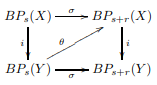
where the top triangle commutes, and the bottom commutes up to a homotopy fixing NP_s(X) - an "r-interleaving"
This tells us that the maps \pi _n(BP_s(X)) \to \pi _n(BP_{s}(Y)) is "almost an isomorphism":
- We can find a preimage for any element in \pi _n(BP_s(Y)), as long as we're willing to increase the allowed error by r. - If two elements in \pi _n(BP_s(X)) agree in \pi _n(BP_s(Y)), they also agree in \pi _n(BP_{s+r}(X))
Let's call something like this an r-isomorphism.
We can then ask in general for an r-equivalence, which gives an r-isomorphism on the (filtered) homotopy groups. These maps have various good properties
- They are stable under composition with weak equivalences - They're not quite stable under composition, rather when composing an r-equivalence and an s-equivalence, you get an r+s-equivalence. - They satisfy a similarly modified version of the 2 out of 3 condition. - A pullback of an r-equivalence which is a fibration is a 2r-equivalence (and a fibration). - If a map is an r-equivalence and a sectionwise cofibration (not the same as a cofibration in the projective model structure!), it admits a 2r-interleaving, in the sense of the diagram above.
This gives a sort of bizzarro model structure/homotopy theory for r-equivalences. In this world, an r-interleaving is a bit like a deformation retract.
Complexity theory, probability [complexity-theory-probability]
- May 2, 2020
-
Eigil Fjeldgren Rischel
Complexity theory, probability [complexity-theory-probability]
- May 2, 2020
- Eigil Fjeldgren Rischel
Computationally bounded probability theory
- May 2, 2020
-
Eigil Fjeldgren Rischel
Computationally bounded probability theory
- May 2, 2020
- Eigil Fjeldgren Rischel
Probability theory is about how to manage incomplete information. One way to interpret a statement like "the probability of event X is p" is in terms of betting odds - you think the probability of X is p if you value a lottery ticket that pays out $1 if X happens at p dollars. From this interpretation, all the laws of probability theory (except arguably those involving infinite conjunctions of events) follow, if we add the requirement that your valuation is "inexploitable" - in other words, if we require that no smart bookie can get you to make a series of bets that always loses money.
The big issue with probability theory as a model of how to reason under uncertain information is that it doesn't account for agents with _limited processing power_ (i.e all of them). A way to think about this problem is that, realistically, the best you can possible hope for is to not be outsmarted by bookies without too much more computing power than you. For example, what is the probability that among the first 10^{10^10} digits of \pi , there are more even than odd ones? If a mortal human is forced to assign this event a probability, we must choose more or less blindly - a bookie with an arbitrarily powerful computer could then win lots of money off us by calculating a lot of inaccessible digits of \pi and betting us for their parity.
This approach to "computationally bounded probability theory" is explored in the paper Logical Induction. Based on the idea about "computationally limited bookies", they build a notion of "logical inductor" - a process which assigns gradually updating probabilities to logical statements, and which is "optimal" in the sense that it can't be exploited.
Computationally bounded logic
- May 2, 2020
-
Eigil Fjeldgren Rischel
Computationally bounded logic
- May 2, 2020
- Eigil Fjeldgren Rischel
In some sense, the problem solved by logical induction is that ordinary logic is _too expressive_. It can express statements which are hard to verify in a small amount of space. Interestingly, there are versions of logic that get around this limitation in various ways. Light Affine Set Theory is a version of set theory with the following interesting property: the provably total functions are precisely those with a polynomial-time algorithm. This means that the function which determines the most common parity among the first 10^{10^n} digits of \pi is _not provably total_ (assuming of course that there is no efficient algorithm for this). Of course, this sort of logic is by necessity much more restricted than normal logic. We can think about this as a sort of ultrafinitism - numbers like 10^{10^n} are "too big to exist".
Synthesis?
- May 2, 2020
-
Eigil Fjeldgren Rischel
Synthesis?
- May 2, 2020
- Eigil Fjeldgren Rischel
What is the unifying thread here? I'm not sure. I want to say something like "you can't prove in LAST that a logical inductor is inconsistent". This is not quite meaningful - a logical inductor is a _sequence_ of probability assignments (as they have more time to calculate, they update their probabilities), and each step along the sequence will generally contain plenty of specific verifiable mistakes. But there's an idea that I'm trying to grasp at, that the inconsistency of a logical inductor "takes superpolynomial resources to detect", and hence it "is" a probability measure from the point of view of a polynomial logic. Or perhaps we should say that it "isn't not a probability measure", in the sense of constructive logic. That is, we can't verify that it's a probability measure, but we can't construct a counterexample either.
The zero-one laws of Kolmogorov and Hewitt–Savage in categorical probability [zero-one-laws-paper]
- April 26, 2020
-
Eigil Fjeldgren Rischel
The zero-one laws of Kolmogorov and Hewitt–Savage in categorical probability [zero-one-laws-paper]
- April 26, 2020
- Eigil Fjeldgren Rischel
TLDR
- April 26, 2020
-
Eigil Fjeldgren Rischel
TLDR
- April 26, 2020
- Eigil Fjeldgren Rischel
This is a post about my paper The zero-one laws of Kolmogorov and Hewitt-Savage in categorical probability, joint with Tobias Fritz. This is a "companion piece" where I try to explain those ideas in a more understandable language. There are essentially three ideas in this paper:
- "Markov categories for synthetic probability theory" - this is only treated briefly, since this is just the background that we're building on top of. Tobias has a long paper on this, A synthetic approach to Markov kernels, conditional independence and theorems on sufficient statistics. - "Kolmogorov products" - a take on tensor products of infinitely many objects. These are introduced into the framework to handle probabilistic systems with infinitely many variables. - "Zero-One Laws". These are theorems from probability theory of the form "If an event A satisfies ..., then P(A) \in 0,1" - i.e either it always happens or it never happens. For two classical ones, Kolmogorov's and Hewitt-Savage's, we give a way of phrasing them in the categorical language and prove them.
In this post, I'll try to give an accessible take on these ideas. I'll assume some familiarity with category theory, and a _very_ small amount of familiarity with probability theory
What do you mean, "synthetic probability theory"
- April 26, 2020
-
Eigil Fjeldgren Rischel
What do you mean, "synthetic probability theory"
- April 26, 2020
- Eigil Fjeldgren Rischel
Synthetic vs analytic
- April 26, 2020
-
Eigil Fjeldgren Rischel
Synthetic vs analytic
- April 26, 2020
- Eigil Fjeldgren Rischel
(This is a weird rambly section. Feel free to skip it)
Think about plane geometry for a moment. Let's contrast two approaches: In the "Euclidean" approach, we work without any reference to what a point, a line, and so on, _is_[^fn:1]. We simply have certain axioms which relate lines and points, certain properties (like congruence) which things can have or not have, and so on. We could also call this approach _formal_, or maybe _syntactical_. We can contrast this with how plane geometry might be treated in the modern world:
- A point is an element of \mathbb {R}^2. - A line is a subset of \mathbb {R}^2 such that ...
and so on. Here a point is really a particular _thing_, so is a line, and the statement "The angle ABC equals the angle CBD" is defined in terms of the things that A,B,C,D are, rather than being a more or less irreducible notion. We call such an approach _analytical_. Another way of looking at it is that Euclidean geometry admits several distinct models (particularly if we abandon certain axioms, e.g. the parallel postulate). On the other hand, the analytical approach of \mathbb {R}^2 augmented with some structure is a _specific_ model.
Markov categories
- April 26, 2020
-
Eigil Fjeldgren Rischel
Markov categories
- April 26, 2020
- Eigil Fjeldgren Rischel
The classical approach to probability theory is analytical - a probability space (\Omega ,\Sigma ,P) is a specific thing with a specific structure. We want to contrast this to a synthetic approach to probability theory. One "model" of our synthetic approach will be "classical probability theory", i.e measures and \sigma algebras. Another model will be given by "possibility theory", where each outcome either happens or doesn't happen. And there are many other exoctic models like that.
This approach is called Markov categories. It is a notion which has been developed by several different authors under different names - see the paper by Fritz above for a review of the literature (and a much more in-depth treatment of Markov categories).
A Markov category is a symmetric monoidal category (\mathsf {C},\otimes ,I), where the monoidal unit is terminal, where each object X \in \mathsf {C} carries a distinguished cocommutative comonoid structure \operatorname {copy}_X: X \to X \otimes X, \operatorname {del}_X: X \to I and such that the symmetric monoidal structure isomorphisms are homomorphisms[^fn:2]. See Tobias' paper for an unpacking of this definition.
The interpretation of a Markov category is that the objects are "spaces" that our random variables can take values in, and the maps are "stochastic processes" or "kernels", i.e functions which produce their output somewhat randomly. The tensor product of two objects X \otimes Y is the "product space" where points are pairs of points (x,y) - but note that this is _not_ a product in the categorical sense, since, give a random map A \to X \otimes Y, we can not in general recover it from the "marginals" or "projections" A \to X and A \to Y. This is because the random values of X and Y may be _dependent_. On the other hand, we do have "diagonal" maps X \to X \otimes X - which non-randomly send x to (x,x) - and a "projection" map X \to I, which is actually unique (there is precisely one way to randomly generate an element of the one-point space).
A map I \to X is called a _distribution on X_, and should be thought of as the abstract version of a probability measure. For instance, if P:I \to X is a distribution, and f: X \to Y is a map, then we can make sense of this diagram:
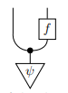
it is the distribution on X \otimes Y where x \in X is sampled according to \psi , then y \in Y is sampled according to f(x). Note the bullet which denotes the copying operator.
We can define a few different standard terms from probability theory in this context.
Independence
- April 26, 2020
-
Eigil Fjeldgren Rischel
Independence
- April 26, 2020
- Eigil Fjeldgren Rischel
Given a map f: A \to X \otimes Y, we can ask whether X,Y are /independent given A /. The intuition here is that given some a \in A, if I sample (x,y) from f(a) and tell you what the x was, that gives you no information about the y (given that you know what the a was). In diagram form, this looks like this:
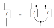
The basic idea here is that it makes no difference whether we generate (x,y) together in one go, or separately (using the same a).
Determinism
- April 26, 2020
-
Eigil Fjeldgren Rischel
Determinism
- April 26, 2020
- Eigil Fjeldgren Rischel
A map f: A \to B is _deterministic_ if we have this equality:
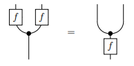
This means if we run f twice with the same a \in A, we get the same b \in B out. This is a reasonable definition of "deterministic".
Note that in both these cases, the existence of the comonoid structure is _exactly_ what we needed to make sense of the probabilistic notion.
Examples
- April 26, 2020
-
Eigil Fjeldgren Rischel
Examples
- April 26, 2020
- Eigil Fjeldgren Rischel
- There is a Markov category \mathsf {Stoch} where the objects are measurable spaces, and the maps are Markov Kernels
- There is a Markov category \mathsf {FinStoch} where the objects are finite sets and the maps are stochastic matrices. It is a full subcategory of \mathsf {Stoch}. - There is a Markov category called \mathsf {SetMulti} where the objects are sets and the maps are "total relations", i.e relations X \to Y where each element x \in X is related to at least one element in Y. - There is a Markov category \mathsf {Gauss} where objects are natural numbers, and maps n \to m are "affine maps \mathbb {R}^n \to \mathbb {R}^m plus constant Gaussian noise"
For (many) more examples, see Tobias' paper.
Infinite tensor products
- April 26, 2020
-
Eigil Fjeldgren Rischel
Infinite tensor products
- April 26, 2020
- Eigil Fjeldgren Rischel
Most theorems in probability theory involve infinite families of variables. To make sense of that in our framework, we need to make sense of "distributions on infinite product spaces", which means we need a notion of "infinite tensor product". The definition goes like this: Let \{X_j\}_{j \in J} be a collection of objects in a markov category \mathsf {C}. For each finite subset F \subset J, we can make sense of the tensor product \bigotimes _{j \in F} X_j[^fn:3]. Since the tensor unit is terminal, we have natural maps \bigotimes _{J \in F'} X_j \to \bigotimes _{j \in F} X_j for each inclusion of finite sets F \subset F'. Then we can ask for a cofiltered limit of this system:
\lim _{F \subset J} \bigotimes _{j \in F} X_jThis is a reasonable definition of "infinite tensor product", which we can denote \bigotimes _{j \in J} X_j However, it turns out we need one more condition. The issue is that in a Markov category, having an object defined up to isomorphism is not always good enough - we want it up to _deterministic isomorphism_, so that the comonoid structure is determined as well. The natural condition to add to make sure we pick the "right" limit is that each of the projections \bigotimes _{j \in J} X_j \to \bigotimes _{j \in F} X_j, for each finite subset, is deterministic. Such an infinite tensor product, we called a _Kolmogorov product_.
Kolmogorov's Zero-One Theorem, abstractly
- April 26, 2020
-
Eigil Fjeldgren Rischel
Kolmogorov's Zero-One Theorem, abstractly
- April 26, 2020
- Eigil Fjeldgren Rischel
With this setup, it turns out it's very easy to prove an abstract version of Kolmogorov's Zero-One Law. Informally, the content of the law is this: suppose you have a family (X_n) of independent random variables, and some event A which is determined by these variables, but is independent of any finite subset of them. Then P(A) \in \{0,1\}
Here is our abstract version: Let (X_j)_{j \in J} be objects so that the Kolmogorov product \bigotimes _{j \in K} exists. Let p: A \to \bigotimes _{j \in J} X_j be a map, and s : \bigotimes _{j \in J} X_j \to T be a deterministic map. Suppose p displays the conditional independence of the X_j given A, and that for every finite F \subset J, the joint distribution
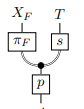
displays the independence of X_F and T given A. (Here X_F = \bigotimes _{j \in F} X_j). Then the composite sp : A \to T is deterministic.
I will sketch the proof (see the paper for details). Essentially, we first prove that T is independent of all the X_j, not just the finite subsets. To see this, we note that the definition of independence is comparing two maps into T \otimes \bigotimes _{j\in J} X_j. This is a limit, so it's enough to show that all the component maps, which are the maps for finite F \subset J, agree - this is true by definition. Now it follows by a string diagram manipulation that sp satisfies the definition of determinism:
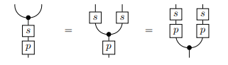
This concludes the proof.
To recover the classical Kolmogorov 0-1 law, we must do a little bit of technical work. We work in the Markov category \mathsf {BorelStoch} of _standard Borel spaces_. This Markov category has countable Kolmogorov products[^fn:4]. We let A = * and let our X_j be the _spaces_ that the variables X_j from the theorem take values in. We let the map p give the joint distribution of the variables. We let T = \{0,1\}, and we let s be the indicator for the event. Then the theorem says that the composite sp is deterministic. So the probability that sp is 1, which is the probability that the event happens, is either zero or one.
[^fn:1]: Euclid actually did try to define notions like lines, points, etc, but we're gonna use his name anyways [^fn:2]: Note that we're not assuming all maps, or even all isomorphisms, are homomorphic. This makes Markov categories an evil notion [^fn:3]: I am handwaving some non-issues with regards to non-strictness here [^fn:4]: It turns out that proving this is significantly harder than proving the abstract theorem, once you have the setup
Bivariate Causal Inference [bivariate-causal-inference]
- April 13, 2020
-
Eigil Fjeldgren Rischel
Bivariate Causal Inference [bivariate-causal-inference]
- April 13, 2020
- Eigil Fjeldgren Rischel
TLDR
- April 13, 2020
-
Eigil Fjeldgren Rischel
TLDR
- April 13, 2020
- Eigil Fjeldgren Rischel
I give a very short introduction to the idea of "causality" in statistics, then talk about two ways to infer causal structure for two variables - i.e, without using conditional independence statements. The ideas here are mostly taken from Peters, Janzing, and Schölkopf: Elements of causal inference: foundations and learning algorithms.
What is causality?
- April 13, 2020
-
Eigil Fjeldgren Rischel
What is causality?
- April 13, 2020
- Eigil Fjeldgren Rischel
A "causal statistical model" is something like this:
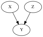
Or this
Where a classical statistical model tells you what the probability of various outcomes are, (which you can then use to derive conditional probabilities, etc), a causal model gives you more information - it tells you how the distribution changes when the system is intervened on. For instance, in the first model above, intervening on X has no effect on the distribution of Z, whereas in the latter, the distribution of Z after the intervention X := x_0 is exactly the conditional distribution P(Z=z|X=x_0).
Causal inference by conditional independence
- April 13, 2020
-
Eigil Fjeldgren Rischel
Causal inference by conditional independence
- April 13, 2020
- Eigil Fjeldgren Rischel
We can actually distinguish between the two causal structures above without doing interventional experiments. This is because in the first model, X and Z are independent, but don't (necessarily) remain independent after conditioning on Y. For instance, if Y = X+Z, learning that Y has a certain value tells us exactly how to compute X and Z from each other. On the other hand, in the second model, X and Z are not (necessarily) independent, but after conditioning on Y, they _are_. That's because the dependency of Z on X only "goes through" Y, so if we already know what Y is, learning about X tells us nothing about Z.
Why are X and Z independent in the first model? This is because of a basic principle of causal modeling, which we can paraphrase as "all (conditional or unconditional) dependencies between variables must be explained by causal structure". (Formally, the distribution has the _markov property_ with respect to the graph).
Bivariate causal inference
- April 13, 2020
-
Eigil Fjeldgren Rischel
Bivariate causal inference
- April 13, 2020
- Eigil Fjeldgren Rischel
We can use conditional (in)dependence to try to tell causal graphs apart. But we can't always do this. For instance, this graph:
Gives rise to exactly the same independence statements as graph 2 above. (We say they are "Markov equivalent"). The worst case is the case where we have just two variables - since both graphs X \to Y and Y \to X are Markov equivalent. (And the third possible DAG, X\ Y, corresponds to the statement that X and Y are independent - not very interesting).
How can we get around this problem, and detect causal structure when we only have two variables? Let's make it concrete, and say that X is a variable that measures whether or not a person smokes, and Y measures cancer. We observe a strong correlation. We have supposed there are no confounding variables, but now we still have the question: does smoking cause cancer, or does cancer cause smoking?
Do an interventional experiment
- April 13, 2020
-
Eigil Fjeldgren Rischel
Do an interventional experiment
- April 13, 2020
- Eigil Fjeldgren Rischel
The easiest way is to just test our theory directly against nature. The difference between the statements X \to Y and Y \to X is whether or not doing the intervention X := x_0 will affect Y or not. In other words, we can take a large number of people, randomly assign them to either smoke or not smoke, then come back a few years later and see whether the smokers have more cancer. This experiment may not get past the ethics board.
Use domain knowledge
- April 13, 2020
-
Eigil Fjeldgren Rischel
Use domain knowledge
- April 13, 2020
- Eigil Fjeldgren Rischel
The idea that cancer causes smoking seems pretty dumb. People generally start smoking, then develop cancer many years later. We could try to build this idea into a more complicated causal model (with more variables), which we could statistically test, but we could also just take seriously the fact that the hypothesis "cancer causes smoking" is prima facie much less plausible than "smoking causes cancer".
These two solutions are both pretty unsatisfying. Fortunately, we also have more sophisticated tools.
Independent mechanisms.
- April 13, 2020
-
Eigil Fjeldgren Rischel
Independent mechanisms.
- April 13, 2020
- Eigil Fjeldgren Rischel
The basic idea is this: if the causal structure is that smoking causes cancer, then whatever process turns smoking into cancer is independent of the process that makes people smoke. This means that learning the conditional distribution P(\mathrm {Cancer}|\mathrm {Smoking}) tells you nothing about the distribution P(\mathrm {Smoking}) itself. On the other hand, learning the smoking rates of cancer victims and non-cancer victims does in fact tell you something about the cancer rate. This is called "The principle of independent mechanisms". The "mechanisms" in question are the distributions P(\mathrm {Smoking}) and P(\mathrm {Cancer}|\mathrm {Smoking}). They are "independent" in the sense that each contains no information about the other. From this principle, we can derive some algorithms for testing the causal relationship.
Semi-Supervised Learning
- April 13, 2020
-
Eigil Fjeldgren Rischel
Semi-Supervised Learning
- April 13, 2020
- Eigil Fjeldgren Rischel
Suppose we try to train a machine learning algorithm to predict whether a person has cancer based on whether or not they smoke. We provide the algorithm with a number of samples (X_i,Y_i), each consisting of a "smoking?" and a "cancer?" measurement. We also provide it with a number of _unlabeled_ samples, X_j, with only the "smoking?" measurement. This is sometimes called "semi-supervised learning". Do these extra samples help the algorithm? The principle of independent mechanisms says "no". These samples only provide information about the distribution P(\mathrm {Smoking}), which gives no information on the conditional P(\mathrm {Cancer|Smoking}). On the other hand, if we're trying to predic smoking from cancer, knowing something about the general cancer rate may actually help. Thus we can try to distinguish X \to Y and Y \to X from each other by seeing whether adding the unlabeled samples helps or not.
Independent noise
- April 13, 2020
-
Eigil Fjeldgren Rischel
Independent noise
- April 13, 2020
- Eigil Fjeldgren Rischel
Linear models are ubiquitous in statistics. A linear model for X \to Y, based on the principle of independent mechanisms, may look like this:
- X := a + bN_1 - Y := c + dX + eN_2 - N_1,N_2 \sim \mathcal {N}(0,1) - N_1,N_2 independent.
In other words, X is normally distributed, then Y is a sum of X times a constant and another normal distribution. The crucial property of this model is the independence of the noise variables. If we run a linear regression to predict Y from X, we will get an error term of (on average) eN_2 - this is independent of X. But in the other direction, we get X = Y/d - c/d with an error term of, on average, \frac {e}{d} N_2 - which is _not_ independent of Y (since Y depends on N_2). Hence we can find the causal direction by running two linear regressions and seeing when we get an independent noise term.
How to Make A Website [2020-02-28-how-to-make-a-website]
- February 28, 2020
-
Eigil Fjeldgren Rischel
How to Make A Website [2020-02-28-how-to-make-a-website]
- February 28, 2020
- Eigil Fjeldgren Rischel
Here's what goes into a website.
- A server (hardware).
- The software which runs on the server, also called a server.
- A domain (optional)
- An SSL certificate (technically optional but highly recommended)
I will explain what these terms mean, and how to get your own stuff set up. Please note that this is a guide for people who want to do everything from scratch. There are plenty of easier ways to set up a website. For instance:
- Any of a number of blogging systems, like wordpress.com, which will also help you hook up your own domain.
- nearlyfreespeech.com - an extremely cheap option if you want to do some things yourself. If your website is just a collection of static pages, this is an easy way to put it on the internet.
How the internet works
- February 28, 2020
-
Eigil Fjeldgren Rischel
How the internet works
- February 28, 2020
- Eigil Fjeldgren Rischel
When you type "reddit.com" into your browser, here's what happens:
- Your computer sends a signal to something called a "DNS server", saying "I need to find 'reddit.com'. Can you tell me where it is?". - Since the people who operate reddit have previously left their address at the DNS server, it says, "yes, you can find it at 151.101.193.140". - Then your computer sends a new message to 151.101.193.140, saying essentialy "I'd like your home page, please" - (if you'd typed in "reddit.com/r/stuff", it would say "I'd like what you have at '/r/stuff', please"). - Your ISP uses those numbers to find the reddit server, which is just a computer running in a warehouse somewhere. - The reddit server sends a message back containing their home page - Your browser displays the page.
Now, what we want to do is the same thing that reddit is doing. So, let's go over the list of things again:
- We need a __domain__, a name for people to find the website. In principle, you can just tell people an IP address like 151.101.193.140, and not use a domain, but that's kind of inconvenient to remember. - Basically, to get a domain, you pay the people in charge of domains some money for ownership of it. Then they write down in the big list of domains that "awesome-website-stuff.xyz" belongs to so and so, and that the IP address is such and such. - (In reality, you buy your domain from an intermediary organization, of which there are many) - We need an actual server, to send the message to people who ask for it. A server is really just a computer - you could "serve" your website from your desktop computer, if you wanted to. In practice, you'll want your server to be running all the time, so it'll probably be easier to rent one. There are many services to do this. - Then you'll need to run a program on the server which can interpret the messages from people who want to see your website and respond with the website. Confusingly, this program is often also called a server. - Lastly, for security reasons, you may want your website in HTTPS. This makes sure the contents of your site are secure. If you'll be sending and receiving information which is not public, this is absolutely essential. Even if you just have a public-facing website with nothing secret on it, setting up HTTPS is a good idea - for instance, it ensures that an attacker can't fake messages from your website, so people can trust that it's really you writing what you put on your website.
Before we proceed, I should mention that I AM NOT A SECURITY EXPERT. If you're going to be handling any sort of sensitive information, please, PLEASE, do some research, and try to consult with someone who knows what they're doing. If you only follow my advice, you should assume that anything you put on your server is immediately compromised.
Server (hardware)
- February 28, 2020
-
Eigil Fjeldgren Rischel
Server (hardware)
- February 28, 2020
- Eigil Fjeldgren Rischel
Basically, we're going to rent a computer from someone for your website to run on. There's a bunch of services to do this, each with their own advantages and problems.
My personal website uses Linode. Their servers start at $5/month for a so-called "nanode". When I need to explain something, I'll use that as the example.
I won't say that I have any great familiarity with the market, so do your own research. The important point for this tutorial is that you get full root access to a server running something like Ubuntu linux.
A lot of services "manage" you in various ways - providing a standardized webserver (as in, __software__ running on your server), limiting the stuff you can do on the server, etc etc. These are not necessarily bad ideas, but it's not what we're looking for.
You can also run whatever OS you want on your server. You'll almost certainly want some variation of Linux. I'll use Ubuntu for this guide. If you're using a different version, things will obviously be different.
- Buy a server somewhere - Set it up to run a recent version of Ubuntu. - Make sure you know the root password of your server (you should be able to view or set this on the website of your provider) - Then find its IP address. - Here's how this looks on Linode:
You can see the IP addresses on the right.
- Do `ssh root@x.y.z.w`, substituting the actual IP address - Log in using the root password
Now you're running a terminal on your server.
Server (software)
- February 28, 2020
-
Eigil Fjeldgren Rischel
Server (software)
- February 28, 2020
- Eigil Fjeldgren Rischel
We're gonna use a program called nginx to serve our website.
- While `ssh`ed into your server, do `apt update` and `apt install nginx` to install nginx. - To start nginx, do `/etc/init.d/nginx start` - To test that it's working, open up a browser and type your ip into the address bar. Your should see a page like this:
Now, I'll explain how to configure nginx to serve your website.
- For this basic tutorial, we'll just set up nginx to serve some .html files in a directory. For a more complicated website, you'll probably want __dynamic__ content, i.e content which is generated by a program running on your server, rather than just read from a file. You can set up nginx to do this, but I won't cover that. - By default, nginx uses the directory `/var/www/` for websites. We're gonna stick with that. Now would be a good time to make up a domain name for your website. Do `mkdir -p /var/www/example.com/html` - Create `/var/www/example.com/html/index.html` using `nano` or another editor. For now, just put this text in it:
<html> <head> <title>Welcome to example.com!</title> </head> <body> <h1>Success! The example.com server block is working!</h1> </body> </html>- Now create the file `/etc/nginx/sites-available/example.com`. Paste this into it:
server{ listen 80; listen [::]:80; root /var/www/example.com/html; index index.html index.htm index.nginx-debian.html; server_name example.com www.example.com; location / { try_files $uri $uri/ =404; } }- Create symlink to this file in the sites-enabled directory: - `ln -s /etc/nginx/sites-available/example.com /etc/nginx sites-enabled/` - nginx is configured by default to serve out of `/var/www/html` - disable the default configuration by doing `rm /etc/nginx/sites-enabled/default` - This will make the directory we've set up the default one. Don't worry, the default configuration file is still available in `sites-available/` - Now test that we didn't fuck up by doing `nginx -t` - this scans the configuration files for errors - Then restart nginx: `systemctl restart nginx.service` - Hopefully going to your server in a browser (by typing in the ip) will now show the page we made.
Obtaining a domain
- February 28, 2020
-
Eigil Fjeldgren Rischel
Obtaining a domain
- February 28, 2020
- Eigil Fjeldgren Rischel
Now let's buy the `example.com` domain.
- As mentioned, there are tons of places to buy a domain. Let's go with hover - Create an account and buy your chosen domain. - Now you'll want to point your domain at the linode server. - When using Linode, the easiest way to do this to use linode's nameservers. - On the Hover control panel, you can see a list of "Nameservers"
- Click edit, and set these to what you see there - `ns1.linode.com` etc - Then log on to Linode, go to "Domains" in the left-hand menu, click "add a new domain", and fill out the information:
(Obviously you'll type in your domain at the top). Note that you __must__ enter an email address.
- The default settings created like this should work. - For reference, here's how mine looks:
- Now you should be able to go to `example.com` or `www.example.com` and see your website. - If you can't, one possibility is that your browser (sensibly) won't let you connect to an unsecured website. We'll fix that now.
HTTPs
- February 28, 2020
-
Eigil Fjeldgren Rischel
HTTPs
- February 28, 2020
- Eigil Fjeldgren Rischel
Now we'll set up security for your site. Luckily, this is super easy.
- `ssh` into your server and do `apt install certbot python3-certbot-nginx` - This installs the auto-setup tool `certbot` from the Let's Encrypt project, as well as the plugin for nginx - Now simply do `certbot --nginx -d example.com -d www.example.com`, and follow the instructions. - Look in `/etc/nginx/sites-available/example.com` - you should see that `certbot` has modified it. - Restart nginx and try to connect to your website.
What now?
- February 28, 2020
-
Eigil Fjeldgren Rischel
What now?
- February 28, 2020
- Eigil Fjeldgren Rischel
Now you're set up! Put any files you want to put on your website into `/var/www/example.com/html`
- Look at the nginx website for more information about configuring it - Use static site generators like Jekyll or Hakyll to generate your website. - Message me to complain about the problems in this guide. - If you buy your domain or your server from somewhere else, they probably have their own guides that tell you how to point your domain at the server. Try googling around.
Frequentist Statistics and Compositionality [2020-02-27-compositional-frequentism]
- February 27, 2020
-
Eigil Fjeldgren Rischel
Frequentist Statistics and Compositionality [2020-02-27-compositional-frequentism]
- February 27, 2020
- Eigil Fjeldgren Rischel
Time-saving blurb: This essay thingy eventually ends without any useful conclusion (I don't manage to figure out how to make something compose). Also, it's not clear that what's here is particularly deep even if it could be made to work, which it hasn't.
P-values
- February 27, 2020
-
Eigil Fjeldgren Rischel
P-values
- February 27, 2020
- Eigil Fjeldgren Rischel
For convenience I'll only work with finite sets - I'm not aware of any serious problems extending this to more general spaces, but it would add some technicalities and it's not really germane to what I'm doing.
Let's say we have a population, and some attribute of the individuals that can be measured - maybe the population consists of humans, and we're measuring their height. Or maybe the population is really "outcomes of an experiment".
The simplest sort of model for something like this is just a probability distribution - a probability p(x) for each possible measurement x. What we want to do is to take some large number of measurements x_1, x_2, \dots x_N, and see if our model is plausible. How to do this? The naive thing would be to calculate the probability of the outcome, which is p(x_1)p(x_2) \cdots p(x_N). For a plausible model, this should be high. One issue is that it's not clear how high is "high enough". Obviously, adding more samples will reduce this towards zero, even for a model that's totally correct. Moreover, if we're looking at a larger set of possibilities, then the probabilities will have to be smaller - again, even if our model is correct.
The classical solution to this question is the "p-value": The probability of getting an outcome which is less or equally likely than the one we actually got. If you think about it, you'll realize that things with higher probabilities also have higher p-values. Moreover, splitting the space of possibilities up doesn't affect the p-value, essentially because it also splits all the lower-probability outcomes up. Taking more samples may increase or decrease the p-value, but tends to decrease it precisely if our model is not exactly right (this is not really trivial). For these reasons p-values are the most ubiquitous way of rating models in statistics. Clasically, we reject a model if the p-value is less than 0.05.
(There are many problems with them, but we won't go into that...)
Open models, rejection relations
- February 27, 2020
-
Eigil Fjeldgren Rischel
Open models, rejection relations
- February 27, 2020
- Eigil Fjeldgren Rischel
Now I want to cook up a categorical/compositional version of this. What's an "open probability distribution"? My best current bet is that it's a stochastic matrix A \to B (where A,B are finite sets). In other words, for each point a\in A, a probability distribution P(b|a) on B. These form a category \mathsf {FinStoch}.
How can I do frequentism to this, in a "compositional" way?. I came up with this definition:
A *plausibility relation* is a function (A \times B)^* \to [0,1]. Here (A\times B)^* is the "Kleene star", the set of finite sequences of pairs (a,b) \in A \times B. The interpretation is that it's a function which sends each sequence to the p-value. Given a stochastic matrix P: A \to B, we can define a plausibility relation p_P((a_i,b_i)_{i=0}^N), to be the probability of observing a sequence of b_is less likely or equally likely to the actual sequence, given that each b_i is distributed according to P( |a_i) (holding the a_is fixed).
Now the puzzle: figure out a composition rule for plausibility relations which makes this into a functor. A reasonable definition could be this:
\[(p \circ q)((a_i,c_i)_{i=0}^N) = \sup_{b_i \in B^N}q((a_i,b_i))p((b_i,c_i))\]This vaguely mirrors the composition rules for relations. Unfortunately it doesn't work.
Basically, the p-value of the least likely outcome is simply its probability (assuming no two outcomes have exactly the same probability), but the formula above isn't the formula for composing stochastic matrices (we should sum instead of taking max). To be completely concrete, let A=B=C = \{0,1\}, let f:A \to B, g: B \to C both be given by flipping the state with probability 1/3. Then the probability of passing from 0 to 1 after both f and g is 4/9, which is also its p-value. The "composite of the p-values" for (0,1) is \max \{p_f(0,1)p_g(1,1), p_f(0,0)p_g(0,1)\} = 1/3.
We could also hope that this construction was a "lax functor", i.e that we always had p_{fg} \geq p_f \circ p_g. This also doesn't hold. Here we can find a counterexample where some outcome c is most likely given a (so has p-value 1), but the most likely b doesn't make c the most likely (so none of the products can be 1). Again, concretely, let A = *, B = \{1,2,3\}, C = \{0,1\}. Define f: A \to B to be 1 with probability 3/7, and both 2 and 3 with probability 2/7. Let g: B \to C be defined so that given 1, it's always 0, and given 2 or 3, it's always 1. Then the most likely outcome is C, so the p-value p_{fg}(*,1) = 1. But for any choice of b, either p_f(*,b) or p_g(b,1) will be less than 1, so the composed p-value can't be one.
Comments
- February 27, 2020
-
Eigil Fjeldgren Rischel
Comments
- February 27, 2020
- Eigil Fjeldgren Rischel
The problem in the last countexample is that the probability is kind of "split up" between 2,3 \in B. This gives them a low p-value, even though we don't care about their difference. But it's not clear that this sort of thinking could be made compositional.