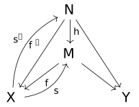
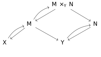
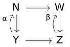
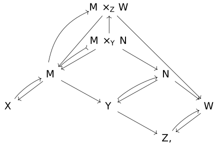
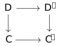
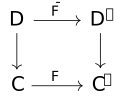
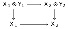
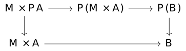
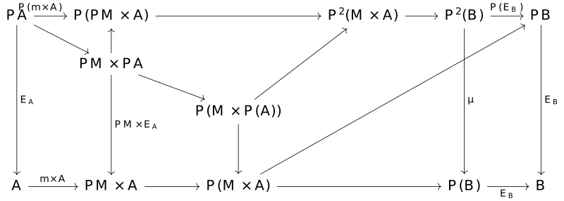
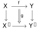
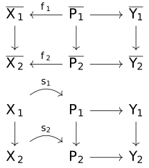
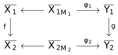
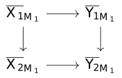
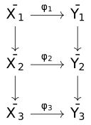
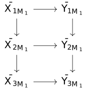
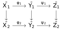
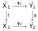
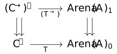
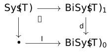
A Markov fibration is a weakening of the notion of (Grothendieck) fibration to include (subject to some assumptions) Markov categories of indexed families of objects (given by deterministic functions E \to X) and compatible stochastic maps (given by commutative squares). The main point of Markov fibrations is that they admit fiberwise opposites, which generalize the fiberwise opposites of ordinary categories. Just as the fiberwise opposite of the codomain fibration of a finitely complete category describes dependent lenses (see § [efr-ZCTD]), the fiberwise opposite of these codomain Markov fibrations give a good notion of stochastic lens (see Theorem [efr-K6NM]).
We will apply our theory chiefly to two problems. First, we will use them to generalize open games (Hedges, Reference [hedges-towards-compositional-thesis]) to a larger class of interfaces (namely, indexed families of sets) while at the same time considering possibly-stochastic maps. This will allow us to construct the so-called external choice operator on open games, which describes branching.
Secondly, we will generalize Myers' categorical dynamical systems theory to allow for stochastic maps in the base. When combined with another generalization of these systems, to general parametrized lenses, this gives a more natural way of modeling certain stochastic dynamical systems, such as those associated to the training dynamics of machine learning models, see eg Example [efr-IMZ3].
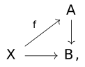
If \mathcal {C} is a category with finite products, the category \mathsf {Lens}(\mathcal {C}) of lenses in \mathcal {C} has objects pairs \binom {A}{X} of objects in \mathcal {C}, and morphisms \binom {A}{X} \leftrightarrows \binom {B}{Y} given by pairs f: X \to Y, f^\#: B \times X \to A. (Note that it is of course the morphisms, not the objects, that are called lenses). One way to generalize this is to ask for \mathcal {C} to have pullbacks, and consider an object given by a more general map A \to X, and let a map be f: X \to Y, f^\#: B \times _Y X \to A (so that the triangle over X commutes). (Note that this recovers the "simple lenses" when the objects are of the form A \times X \to X). Under the interpretation of a map A \to X as a family of objects A_x indexed over the elements of X, we see this as a "dependent lens" (since A is a "dependent type"). There are various variations of this idea, which ultimately all fit the pattern of taking a Grothendieck fibration \mathcal {D} \to \mathcal {C} and forming the fiberwise opposite---for the dependent lenses as above, this is the codomain fibration \mathcal {C}^\to \to \mathcal {C}.
Meanwhile, another wide-ranging generalization of \mathsf {Lens}(\mathcal {C}) are the optics of Riley (Reference [riley-optics]). For \mathcal {C} a monoidal category, the objects of \mathsf {Optic}(\mathcal {C}) are again pairs \binom {A}{X} of objects, but now the morphisms are elements of the coend \int ^{M \in \mathcal {C}}\mathcal {C}(X, M \otimes Y) \times \mathcal {C}(M \otimes B, A). That is, to give an optic \binom {A}{X} \leftrightarrows \binom {B}{Y} is to give an object M \in \mathcal {C} and morphisms l: X \to M \otimes Y, r: M \otimes B \to A, up to the equivalence relation generated by, whenever s: N \to M, l: X \to N \otimes Y, r: M \otimes B \to A, identifying the two optics given by (M, (s \otimes 1_Y) \circ l, r) and (N, l, r \circ (s \otimes 1_B)). One can show that, in the case where \mathcal {C} is a Cartesian monoidal category, this set can be identified with the set of (simple) lenses.
A vector field on a smooth manifold X is simply a (smooth) section of the tangent bundle TX.
A section is a bundle map from the trivial bundle X \to X. This gives the idea of considering a parametrized dynamical system as consisting of a map X \to A to some other smooth manifold, a bundle E \to A (the points of E are the parameters) and a bundle map E \times _A X \to TX.
As we will see, such a bundle map is exactly a dependent lens in a category of bundles. Building on this idea, Myers (Reference [myers-cst]) described a highly abstract theory of open dynamical systems, given by lenses out of tangent bundles (where the notion of space, bundle and tangent bundle are generalized to any fibration).
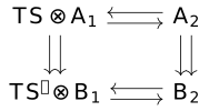
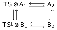
It has been observed that, although a lens from the tangent bundle TS \leftrightarrows A may indeed be said to describe an open dynamical system with state space S, the same can be said for a lens of type TS \otimes A \leftrightarrows I---although a dynamical system of a different kind (essentially, the first type are the Moore machines, the second the Mealy machines---see the introduction to § [efr-000D] for more on this). It is natural to consider parametrized maps TS \otimes A \leftrightarrows B as a common generalization of these two concepts---and in fact, special cases of this idea, lenses parametrized by tangent bundles, have already been considered many times, for example in the semantics of gradient descent (see Reference [bruno-etal-categorical-learning-2021], Reference [towards-cybercat], Reference [backprop-as-functor]).
Since parametrized maps compose in an obvious way, we now have three different notions of morphisms between bundles---lenses, charts, and "generalized systems". These should form some sort of symmetric monoidal triple category, but the right axiomatisation of this concept is somewhat elusive.
Lenses, in their various incarnations, have been widely used in applied category theory. For example, Hedges and his collaborators have developed a compositional approach to game theory (Reference [hedges-string-games], Reference [hedges-etal-comp-gametheory], Reference [hedges-etal-institutions], Reference [hedges-etal-graph-games], others). Recent work by Hedges and Sakamoto bring this idea to reinforcement learning (Reference [sakamoto-reinforcement-lenses]). We briefly mentioned Myers' categorical systems theory above, and we will see much more of it later. As we discussed above, there is also a literature using lenses to study gradient descent in an abstract sense. This is without even mentioning their original role in the theory of functional programming (this is the origin of the somewhat confusing term lens), or their prehistory in Gödel's dialectica interpretation---see eg Reference [jules-lenses-blogpost] for a survey of this.
An open game, in the sense of Hedges, has as its interface two objects in the category of lenses (of sets) \binom {S}{X}, \binom {R}{Y} (that is, two pairs of sets). An open game with this interface consists of a set \Sigma of strategies equipped with a function \Sigma \to \mathsf {Lens}(\mathsf {Set})(\binom {S}{X},\binom {R}{Y}), and a subset Eq(x, k) \subset \Sigma of equilibrium strategies for each x \in X and k: Y \to R---note that such an x is exactly a lens \binom {*}{*} \leftrightarrows \binom {S}{X}, and such a k is exactly a lens \binom {R}{Y} \to \binom {*}{*}. This view of open games makes the composition rule much simpler to define, although we will not delve into the details here, see eg Reference [hedges-etal-comp-gametheory]. The idea is that the open game represents the strategies and preferences of a player or set of players---\sigma \in \Sigma are the possible strategies, x \in X is the information revealed to the player before they make their decision of which moves to make, the resulting y \in Y is the choice the player "sends" in response to x, and the r \in R is the "utility", the value they eventually learn, depending on their choice y, which they have some preferences over.
The above description gives a theory of deterministic games, but of course, it is completely essential for game theory to model both random decisions (mixed strategies) and decisions made under uncertainty. This motivates the replacement of lenses in this definition with optics in a category of probability kernels (the form of the equilibrium relation must be modified as well, see Reference [hedges-etal-bayesian-games], Reference [towards-cybercat])
In the abstract study of open games, it is desirable to define a "choice" operation \oplus on the objects (the pairs of sets) so that maps into \binom {R}{X} \oplus \binom {R'}{X'} represent players who are faced with some binary choice between X and X', after which play may proceed for a time in one of two branches. However, this is immediately problematic because the category of lenses do not have coproducts---inside the category of dependent lenses, however, we can form the coproduct simply as R \times X + R' \times X' \to X + X'---that is, we get a family which is R over X, and R' over X'. This indeed does the job, but for game theory the extension to stochastic maps---optics---is absolutely essential. This motivates the search for a theory of dependent optics, a common generalization of optics and dependent lenses.
There have been a number of attempts at this---see eg Reference [fibre-optics-2021], Reference [hedges-braithwaite-dep], Reference [milewski-polylens], Reference [vertechi-dep-optics]. While these efforts have to some extent succeeded in describing a theory that is general enough to contain the desired examples, it is generally very ad hoc. The construction of optics as a special case of Vertechi's dependent optics (Reference [vertechi-dep-optics]) gives them as fibre optics with the indexing bicategory being (the delooping of) a monoidal category \mathcal {M}, but embeds lenses using a bicategory of spans. Thus simple lenses admit two distinct encodings in this theory. Moreover, Vertechi's example of dependent monoidal optics fails to describe a supercategory of \mathsf {Optic}(\mathcal {C}) when applied to Markov categories, and are thus not suitable for, for example, game theory.
The observation that both open games and machine learning systems can be fruitfully described using lenses, naturally led to the idea that this could be used to develop a more thorough analogy between the two. After all, a machine learning system is also a player in a kind of game (with the objective of minimizing loss). Hedges coined the phrase categorical cybernetics to describe this locus of ideas (Reference [towards-cybercat], also used in Reference [sakamoto-reinforcement-lenses]).
Myers' categorical systems theory also describes dynamical systems as lenses. However, where a cybernetic system in the sense of Reference [towards-cybercat] is a parametrized lens \Sigma \otimes {\bar {X} \choose X} \leftrightarrows {\bar {Y} \choose Y}, and thus has two different inputs - x \in X, which is the information on which basis they are allowed to choose their decision y \in Y, and y^\sharp \in \bar {Y}, which is their "utility", the information they are allowed to care about.
It is straightforward to describe the machine learning part of the categorical cybernetics analogy in terms of Myers' theory---a "learner" is simply a lens of the above form with \Sigma replace with a tangent bundle TS. This idea (described in these terms, although not with the analogy to machine learning) has already been described by Reference [energy-driven-systems].
However, for game theory, it is necessary that the output of a given system can be stochastically chosen (a player must be able to randomize their strategy). At the same time, for a machine learning system, the x \in X is usually some sort of sample from a training distribution---ie, it is random. Hence to really describe the training dynamics of machine learning systems using this theory, we are again naturally drawn to consider systems theories (that is, fibrations) which have stochastic maps in the base, not merely the fiber.
We begin the thesis in § [efr-POD2] with a review of some preliminary material. This chapter can largely be skipped for readers already familiar with the material (Markov categories, double categories, lenses and optics, fibrations, and categorical dynamical systems theory). The chapter on Markov categories introduces a few novel auxiliary notions, but these can be referred back to as necessary (they are primarily regularity conditions which hold in most Markov categories of interest).
In § [efr-O088], we give the main technical contribution of the thesis by developing a theory of Markov fibrations. Their fiberwise opposites generalize both the fiberwise opposites of codomain fibrations (dependent lenses in a classical sense) and optics in Markov categories. Theorem [efr-K6NM] provides the statement of the latter (the former is straightforward). We also give a description of monoidal structures on Markov fibrations (which pass to monoidal structures on the resulting categories of optics).
In § [efr-000D], we give a construction of the double category of parametrized morphisms for a category action (or actegory)---in fact, we do this internally to any 2-category. This has the advantage of allowing us to construct more highly-structured versions of this double category by carrying out the construction internally to higher-structured actions. (Bicategorical versions of \mathsf {Para} are a relatively old idea, and the double categorical version is a straightforward extension which has existed for some time as folklore, but the fully-internal construction here is novel).
In § [efr-GFG0], we apply Markov fibrations to compositional game theory, and solve a longstanding problem by giving a category of stochastic open games with a general "external choice" operator. This construction is largely abstract over the particular category, and so can be applied to different Markov fibrations to describe games defined with different notions of stochasticity. We also review some previous work with Capucci, Hedges, and Gavranovic on abstract constructions of categories of open games (Reference [towards-cybercat]).
In § [efr-ZRUZ], we describe how to extend Myers' categorical systems theory to Markov fibrations, to give theories of systems which may have stochastic maps not merely in the fiber (as was already described by Myers in Reference [myers-cst]) but also in the base. We also leverage our construction from § [efr-000D] to give a description of a symmetric monoidal triple category whose three types of morphisms, are lenses, charts, and what we call bisystems, that is morphisms TS \otimes A \leftrightarrows B - these are open dynamical systems which have two directions of interaction with the environment.
We also describe a particular systems theory of smooth manifolds and smooth stochastic maps between them.
I would like to extend a great thanks to the Mathematically Structured Programming group at the University of Strathclyde, my fellow PhD students in particular, for making my time there such a great one. A good chunk of this work was completed while I worked at the Compositional Systems Laboratory at the Tallinn University of Technology---I owe everyone there a great thanks as well.
For conversations which contributed to this work, and to my mathematical development in general, I would like to thank Dylan Braithwaite, Matteo Capucci, Elena di Lavore, Tobias Fritz, Davidad, Tomáš Gonda, Bruno Gavranović, Diana Kessler, Owen Lynch, Jade Master, David Jaz Myers, Riu Nakamura, Chad Nester, Evan Patterson, Paolo Perrone, Mario Roman, Brandon Shapiro, Toby Smithe, Pawel Sobocinski, David Spivak, and Andre Videla. A special thanks to Dylan, Matteo, and Bruno, for serving their time with me in the dependent optics mines.
To Neil Ghani, Radu Mardare, and Jules Hedges, a massive thanks for serving as my advisors during the somewhat tumultuous process that was the production of this thesis.
Finally, I thank my wonderful family. Now you can stop asking me about it.
We will begin by reviewing some theory that plays a key role in this thesis. With a very few exceptions, nothing here is novel, but we find it useful to include these here---both for the convenience of the reader, to familiarize them with theory that we will make constant reference to, but also to set the stage for our contributions.
First, the theory of (Grothendieck) fibrations. There is far too much to say about these for such a brief space, so we will limit ourselves to what we need for the rest of the thesis, especially for the section on Markov fibrations.
Second, we will give an overview of optics and lenses, in a bit more detail than the introduction. We have already given a review of the sources there, but we will find it useful to put this on proper footing.
Next, we will review the theory of Markov categories. This is a synthetic approach to probability theory, introduced by Fritz Reference [fritz-synthetic-markov-cats], and since developed further by many collaborators, including the author. Here we note the only exceptions to the claim that nothing in this chapter is novel. First, the notion of representable Markov categoryDefinition [efr-38FR] was introduced by Fritz, Gonda, Perrone, and the author in Reference [fritz-gonda-perrone-rischel-rep]. We will not give a thorough treatment here, but since representable Markov categories are so ubiquitous, we will frequently note how different properties or structure on a Markov category relates to representability. We will also introduce a few new concepts which play a role in the theory of Markov fibrations in § [efr-O088]. These are of no great independent interest, as far as we can tell, nor are they difficult, but this seemed the best place to put them.
Finally, we give a brief review of Myers' categorical systems theory. This will mainly be to set the stage for § [efr-ZRUZ], where we develop a triple categorical version of the theory.
In category theory, there are many families of categories indexed by the objects of some other category. For example, for each commutative ring, we have the category \mathsf {Mod}(R).
Given a ring homomorphism \phi : R \to S, there is an induced restriction of scalars functor \phi ^*: \mathsf {Mod}(S) \to \mathsf {Mod}(R) (given simply by composing the module structure by \phi ), and this is (contravariant) functorial, assembling into a functor \mathsf {Mod}(-): \mathsf {CRing}^\mathrm {op} \to \mathsf {Cat}.
In most cases, one can not expect strict functoriality as above. From an abstract point of view, it makes sense that one should really ask only for a natural isomorphism \phi ^*\psi ^* \simeq (\psi \phi )^*, up to some coherence conditions. This assembles into a so-called pseudofunctor into the 2-category \mathsf {Cat}.
From a concrete point of view, there are many natural families of categories which arise as pseudofunctors. For example, restriction of scalars always has a left adjoint (extension of scalars, given by M \mapsto M \otimes _R S, viewing S as an R-module via the map \phi )---since adjoints compose (that is, if F \vdash G and F' \vdash G', then FF' \vdash G'G) this must be functorial up to natural isomorphism, but this is the best we can promise.
To avoid the higher categorical algebra involved in working with pseudofunctors, Grothendieck introduced the notion of fibration in Reference [grothendieck-descent-fibrations].
Let p: \mathcal {D} \to \mathcal {C} be a functor. Given X \in \mathcal {C}, write \mathcal {D}_X for the (strict) pullback \{x\} \times _\mathcal {C} \mathcal {D}. Explicitly, this consists of the objects in \mathcal {D} with p(A) = X and the morphisms with p(f) = 1_X.
Let f: X \to Y \in \mathcal {C} be a morphism.
A map \bar {f}: \bar {X} \to \bar {Y} with p(\bar {f}) = f is locally Cartesian if for each \bar {X}' with p(\bar {X}') = X, postcomposition with \bar {f} induces a bijection
\{g: \bar {X}' \to \bar {X} \mid p(g) = 1_X\} \xrightarrow {\sim } \{g' : \bar {X'} \to \bar {Y} \mid p(g') = f\}
A map is Cartesian if for every g: Z \to X and \bar {Z} with p(\bar {Z}) = Z, there is a bijection
\{\bar {g} : \bar {Z} \to \bar {X} \mid p(\bar {g}) = g\} \to \{\bar {g}' : \bar {Z} \to \bar {Y} \mid p(\bar {g'} = fg)\},
note that every Cartesian map is locally Cartesian (take g = 1_X)
p is a Grothendieck fibration (or just fibration) if, for every \bar {Y} \in \mathcal {D} such that p(\bar {Y}) = Y, there exists a Cartesian map \bar {f}: \bar {X} \to \bar {Y} (for some \bar {Y}) so that p(\bar {f}) = f
p: \mathcal {D} \to \mathcal {C} is a Grothendieck fibration if and only if every f admits a locally Cartesian lift, and the class of locally Cartesian morphisms in \mathcal {D} is stable under composition.
Let \mathcal {D} \to \mathcal {C} be a Grothendieck fibration. For every f: X \to Y, \bar {Y} \in \mathcal {D}_Y, select a Cartesian lift f^*\bar {Y} \to \bar {Y} of f.
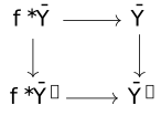
Then there is a unique extension of f^* to a functor \mathcal {D}_Y \to \mathcal {D}_X so that the squares
commute. With this, the assignment X \mapsto \mathcal {D}_X, f \mapsto f^* assembles into a pseudofunctor \mathcal {C}^\mathrm {op} \to \mathsf {Cat}.
If \mathcal {D} \to \mathcal {C} is such that each morphism admits merely a locally Cartesian lift (but these do not compose,) it is called a prefibration. Note that this is unrelated to our notion of Markov prefibration (reading ahead a bit, the "Cartesian" maps in a Markov prefibration do compose, but they enjoy the unique lifting property only for a subset of morphisms). This clash of terminology is perhaps unfortunate, but other potential prefixes seemed inferior (quasi-, pseudo-, semi-).
Let \mathcal {C} be any category, and let \mathcal {C}^\to denote the arrow category. Then the codomain functor \mathcal {C}^\to \to \mathcal {C} is a fibration if and only if \mathcal {C} admits all pullbacks, and in this case the functors f^*: \mathcal {C}_Y \to \mathcal {C}_X, given f: X \to Y, are given by pullback along f.
The functors f^* are sometimes referred to as pullback, a convention we generally adopt. They are also sometimes called base-change functors.
When f: X \to Y and A \in \mathcal {D}_Y, we may write A_X for the object f^*A if there is no chance of confusion. (Compare that the choice of f is also suppressed in the notation A \times _Y X for a pullback)
We will not go into a comprehensive description of the theory of fibrations, but simply give a few basic results. We will give some examples in the next section. For a textbook treatment, see eg. Reference [jacobs-categorical-logic] (chapters 1, 9), or Reference [borceux-handbook] (chapter 8). Note that we will not give a formal definition of the term "pseudofunctor" here. See eg Reference [jacobs-categorical-logic], def. 1.4.4.
Let \mathcal {A}: \mathcal {C}^\mathrm {op} \to \mathsf {Cat} be a pseudofunctor. Then there is a category \int _{X \in \mathcal {C}}\mathcal {A}(X) defined as follows:
The objects are pairs {\bar {X}\in \mathcal {A}(X) \choose X \in \mathcal {C}}
The morphisms {\bar {X} \choose X} \to {\bar {Y} \choose Y} are pairs f: X \to Y, f^\#: \bar {X} \to \mathcal {A}(f)(\bar {Y}) \in \mathcal {A}(X)
Composition is given by the "chain rule" (f,f^\#) \circ (g,g^\#) = (fg, \mathcal {A}(g)(f^\#)g^\#)
There is an obvious forgetful functor \int _X \mathcal {A}(X) \to \mathcal {C}.
The category \int _X \mathcal {A}(X) is known as the Grothendieck construction of \mathcal {A}
Given f: X \to Y and \bar {Y} \in \mathcal {A}(Y), it is clear that the map {\mathcal {A}(f)(\bar {Y}) \choose X} \to {\bar {Y} \choose Y} given by f, 1_{\mathcal {A}(f)(\bar {Y})} is locally Cartesian---the required bijection is the definition of maps in the Grothendieck construction. But it's straightforward to see that these compose.
Given a pseudofunctor \mathcal {A}: \mathcal {C}^\mathrm {op} \to \mathsf {Cat}, it is obvious that the assignment \mathcal {A}(-)^\mathrm {op} is pseudofunctorial as well (the required natural isomorphisms are just the formal opposites of the ones for \mathcal {A}). Applying this through the equivalence of fibrations and pseudofunctors leads to the fiberwise opposite of a fibration. Explicitly:
Let p: \mathcal {D} \to \mathcal {C} be a fibration.
Then there exists a category \mathcal {D}^\mathrm {fop}, called the fiberwise opposite of \mathcal {D}, whose objects are the same as \mathcal {D}, and where a morphism X \to Y is a tuple (f: p(X) \to p(Y), f^\#: f^*Y \to X \in \mathcal {D}_{p(X)}).
We have already given somewhat of an account of lenses, optics, and their applications in the introduction. We briefly review the theory here, especially to normalize the notation and definitions. The best general source for this material is still Reference [riley-optics].
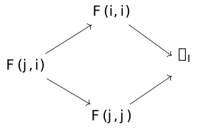
The definition of optic relies on the notion of coend, which we briefly recall, see Reference [fosco-coend-calculus] for a textbook account. If F: \mathcal {I}^\mathrm {op} \times \mathcal {I} \to \mathcal {C} is a functor, the coend\int ^{i \in I} F(i,i) is defined as the initial object receiving a map f_i : F(i,i) \to \int ^{i \in I} F(i,i) for each i \in I, so that for each \phi : i \to j, the square
commutes.
If \mathcal {C} has enough colimits, we may express the coend as the coequalizer of the diagram
\coprod _{f : i \to j \in \mathcal {I}} F(i,j) \rightrightarrows \coprod _{i} F(i,i),
where the two maps are given on each component by F(i,f): F(i,j) \to F(i,i) and F(f,j) : F(i,j) \to F(j,j), respectively. (This is Remark 1.2.4 in Reference [fosco-coend-calculus]). Note that in particular this implies that if \mathcal {C} has all colimits, then it also has all coends.
Let \mathcal {M} be a monoidal category which acts on two categories \mathcal {C}, \mathcal {D}. Then the category of optics\mathsf {Optic}_\mathcal {M}(\mathcal {C},\mathcal {D}) has
The set of morphisms {A \choose X} \to {B \choose Y} given by the coend
\int ^{M \in \mathcal {M}} \mathcal {C}(X, M \cdot Y) \times \mathcal {D}(M \cdot B,A)
Given two optics with representatives (M,f: X \to M \cdot Y,g : M \cdot B \to A), (N, f': Y \to N \cdot Z, g': N \cdot C \to B), their composite is given
by (M \otimes N, (1_M \cdot f')f, g (1_M \cdot g')), where we omit coherence morphisms.
When \mathcal {C} is a monoidal category acting on itself by tensor, we write \mathsf {Optic}_\mathcal {C}(\mathcal {C},\mathcal {C}) =: \mathsf {Optic}(\mathcal {C})
Note that if \mathcal {M},\mathcal {C},\mathcal {D} are symmetric monoidal and these actions are symmetric, \mathsf {Optic}_\mathcal {M}(\mathcal {C},\mathcal {D}) inherits a symmetric monoidal structure given by {A \choose X} \otimes {B \choose Y} = {A \otimes B \choose X \otimes Y}. (Also given a braiding one can induce a non-symmetric monoidal structure, but this almost never comes up).
Objects and morphisms in the category of optics have two parts---one going "forwards", in the same direction as the optic, and one going "backwards". In Reference [riley-optics] the objects are written (X,A), where X is the forwards part. Hedges' work on open games used the binomial notation \binom {X}{A}, but wrote the forwards part on top.
To make the connection to fibrations more natural, we instead write the forwards part on the bottom, {A \choose X}. It is the backwards part which depends on the forwards part, hence the forwards part is the base of the fibration (when one exists)---and every part of the language of fibrations is built around a mental model where the base is at the bottom and the fibers are over it (including the word "base"). When reading the references, this may cause some confusion, but hopefully this can be overcome.
While we're at it, let us note that when talking about optics we will freely use terms like "the forwards part" "the backwards object" and so on---the meaning of this should now be clear. Of course, once we get to cooptics/charts, this would be more than a little confusing, since in that case both components are in the same direction. In those cases we will speak of either the primary (forwards) part or the secondary (backwards) part, or use the language of fibrations and speak of the map or object "in the base" and "in the fiber".
As noted above, the coend \int ^M \mathcal {C}(X, M \cdot Y) \times \mathcal {D}(M \cdot B, A) consists of triples (M, f: X \to M \cdot Y, g: M \cdot B \to A) up to the equivalence relation which, for every \phi : M \to M', f: X \to M \cdot Y, g: M' \cdot B \to A, identifies the two tuples (M', (\phi \cdot 1_Y) f, g) and (M, f, g (\phi \cdot 1_B)). Note that this relation is not assumed to be inherently an equivalence relation---one takes the transitive-symmetric closure as usual.
We call this relation the sliding relation (because we slide the map \phi from the backwards part to the forwards part).
Suppose \mathcal {M}, \mathcal {C}, \mathcal {D} are small categories. Then the coend defining \mathsf {Optic}_\mathcal {M}(\mathcal {C},\mathcal {D})\left ( {A \choose X}, {B \choose Y} \right ) is a small colimit of small sets, hence again small. Since clearly the set of objects \operatorname {\mathbf {ob}} \mathcal {C} \times \operatorname {\mathbf {ob}} \mathcal {D} is small, \mathsf {Optic}_\mathcal {M}(\mathcal {C},\mathcal {D}) is again a small category.
However, if \mathcal {M},\mathcal {D},\mathcal {C} are merely assumed to be locally small, we can not guarantee the same is true of \mathsf {Optic}_\mathcal {M}(\mathcal {C},\mathcal {D}), since the hom-sets are now defined by a coend/colimit with large indexing category. However, in many special cases, it can still be seen to be locally small, such as in the Cartesian case (where \mathsf {Lens}(\mathcal {C}) is clearly locally small).
In this thesis, we will not delve further into this subtlety, simply working inside some universe where all our categories are small.
Of course, we can also let the arrows in \mathcal {D} go in the same direction as \mathcal {C}. This does not seem to have played any role in the literature, but we will give this a name, as it is a useful example to have in mind for Markov fibrations (where we will construct our dependent optics, conceptually, as a fiberwise opposite)
Given \mathcal {M} acting on \mathcal {C}, \mathcal {D}, the category of co-optics, \mathsf {coOptic}_\mathcal {M}(\mathcal {C},\mathcal {D}) has objects pair {A \in \mathcal {D} \choose X \in \mathcal {C}}, and morphisms given by the coend \int ^M \mathcal {C}(X, M \cdot Y) \times \mathcal {D}(M \cdot A, B)
For any monoidal category \mathcal {C}, \mathsf {Optic}_\mathcal {C}\left ({A \choose X}, {I \choose I}\right ) = \mathcal {C}(X,A). One way to think of an optic {A \choose X} \leftrightarrows {B \choose Y} is as a string diagram X \to A, but which has a hole with space for a morphism B \to Y. One inserts such a morphism by composing the optic with the optic {B \choose Y} \leftrightarrows {I \choose I} representing it. This idea of "open diagrams" has been developed in much more detail by Román, Reference [roman-optics-coend].
Suppose \mathcal {M} is semicartesian---in other words, that I \in \mathcal {M} is terminal. Then there is a functor \mathsf {Optic}_\mathcal {M}(\mathcal {C},\mathcal {D}) \to \mathcal {C}, which takes a {A \choose X} to X, and pair \langle f: X \to M \cdot Y, g \rangle to the composite X \to M \cdot Y \to I \cdot Y \cong Y.
In the case of \mathsf {Optic}(\mathcal {M}), the map \mathsf {Optic}(\mathcal {M})({I \choose I}, {A \choose X}) \to \mathcal {M}(I,X) is a bijection.
The fact that in \mathsf {Optic}(\mathcal {M}), states (maps from the monoidal unit) on {A \choose X} are given by states on X, while costates are given by maps X \to A plays an important role in the use of optics to describe open games. See § [efr-GFG0] for more on this.
Here we use a general fact about coends, that \int ^M \mathcal {C}(X,M) \times F(M) \cong F(X)---this has been called the ninja Yoneda lemma, see Reference [fosco-coend-calculus].
In this case we sometimes write \mathsf {Lens}(\mathcal {C}) for the category \mathsf {Optic}(\mathcal {C}). We have the following fact:
The functor {A \choose X} \mapsto X, \mathsf {Lens}(\mathcal {C}) \to \mathcal {C}, is a fibration. The fiber \mathsf {Lens}(\mathcal {C})_X has the following description:
Its objects are the objects of \mathcal {C}.
A map A \to B \in \mathsf {Lens}(\mathcal {C})_X is a map X \times B \to A \in \mathcal {C}.
The composite of X \times B \to A,X \times C \to B is given by composing the two into X \times X \times C \to A, then using the diagonal.
Given f: X \to Y, the pullback functor \mathsf {Lens}(\mathcal {C})_Y \to \mathsf {Lens}(\mathcal {C})_X is given by precomposing by f.
If \mathcal {C} moreover admits pullbacks, there is a fibred functor \mathsf {Lens}(\mathcal {C})^\mathrm {fop} \to \mathcal {C}^\to \to \mathcal {C}, which carries an object {A \choose X} to X \times A\xrightarrow {\pi _X} X, and a morphism f:X \times A \to B to the map X \times A \xrightarrow {\langle \pi _X,F \rangle } X \times B over X. This is fully faithful.
This is the first way to see the maps of (\mathcal {C}^\to )^\mathrm {fop} as dependent lenses---they receive the category of lenses as a full subcategory.
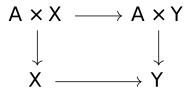
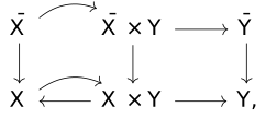
The squares
are pullbacks in any category with products, even if it does not admit pullbacks in general.
It follows that the full subcategory of \mathcal {C}^\to spanned by objects of this form is always a fibration over \mathcal {C}, which is isomorphic to \mathsf {coOptic}(\mathcal {C})---the fiberwise dual is isomorphic to \mathsf {Lens}(\mathcal {C}).
The basic idea of a Markov category is to interpret morphisms X \to Y as "stochastic processes" or kernels---that is, functions valued in probability measures. A morphism P \to X \otimes Y is a parametrized joint probability measure---the comonoid structure allows us to build a canonical such given parametrized measures P \to X, P \to Y (by precomposing their tensor with the \mathrm {copy}_P map). This is the product measure of the two---the fact that in general not every map has this form (because \mathcal {C} is not necessarily Cartesian) allows us to express the probabilistic dependence---as in, non-independence---of one variable on another.
A morphism is called deterministic if it is a comonoid (co)homomorphism, which amounts to the claim that \mathrm {copy}_Y f = (f \otimes f) \mathrm {copy}_X---in other words, that running two independent copies of the kernel (with the same input) is equivalent to running one and copying the output. The deterministic morphisms form a Cartesian monoidal subcategory which is denoted \mathcal {C}_\mathrm {det} \subseteq \mathcal {C}.
We first note the following alternative characterization of Markov categories in terms of their deterministic morphisms.
Let \mathcal {C} be a symmetric monoidal category. A premarkov structure on \mathcal {C} is a wide symmetric monoidal subcategory \mathcal {C}' \subseteq \mathcal {C}---that is, a class of morphisms which contains all identities and structural isomorphisms, and is stable under composition and monoidal products---so that the monoidal category \mathcal {C}' is Cartesian.
Given a premarkov structure\mathcal {C}' \subseteq \mathcal {C}, there is a unique Markov structure on \mathcal {C} so that each morphism in \mathcal {C}' is deterministic.
Given a Markov structure, \mathcal {C}_\mathrm {det} \subseteq \mathcal {C} is a premarkov structure.
A premarkov structure has the form \mathcal {C}_\mathrm {det} for some Markov structure if and only if it is maximal.
The existence part first claim is clear: \mathcal {C}' acquires a unique Markov structure since it is Cartesian, and the inclusion of that Markov structure into \mathcal {C} gives a Markov structure on \mathcal {C}. Conversely, suppose \mathcal {C} is a Markov category and \mathcal {C}' \subseteq \mathcal {C}_\mathrm {det} is a class of deterministic morphisms which is still Cartesian. This means the projections X \otimes Y \to X,Y still exhibit X \otimes Y as a product in \mathcal {C}'. But since the pairing are the unique map lifting two given maps A \to X,Y, the pairing must be preserved by the inclusion \mathcal {C}' \to \mathcal {C}_\mathrm {det}. Since the canonical Markov structure is given as a pairing, this means the markov structure induced by \mathcal {C}' \to \mathcal {C} must agree with the one given by \mathcal {C}_\mathrm {det}, which is just the original one.
Now suppose \mathcal {C}_\mathrm {det} \subseteq \mathcal {C}' \subseteq \mathcal {C}, where \mathcal {C}' is some larger premarkov structure. By the argument above, they must generate the same Markov structure on \mathcal {C}. But again, this implies that every map in \mathcal {C}' is deterministic for this Markov structure, so we have \mathcal {C}_\mathrm {det} = \mathcal {C}'. This finishes the proof.
Note that given a merely monoidal category, we can ask whether it is Cartesian, and if it is, it admits a unique symmetry induced by the universal property of the product. Hence if \mathcal {C}' \subseteq \mathcal {C} is a Cartesian wide monoidal subcategory, we may attempt to define a symmetry on \mathcal {C} simply using the one from \mathcal {C}'. However, it is not automatic that this symmetry is natural for all the morphisms in \mathcal {C}.
This basic idea was already noted by Fritz (and goes back to Golubtsov's work in Reference [golubtsov-kleisli], an important part of the prehistory of Markov categories), although the precise statement above appears to be novel. Since the coherence conditions required of the comonoids in a Markov structure can be somewhat hard to remember, this characterization may be easier to understand.
A Markov category is representable if the inclusion \mathcal {C}_\mathrm {det} \hookrightarrow \mathcal {C} admits a right adjoint. In this case we denote the right adjoint P and call the object PX for X \in \mathcal {C} a distribution object for X. Observe that \mathcal {C}(X,Y) = \mathcal {C}_\mathrm {det}(X,PY) (by definition,) and hence \mathcal {C} = Kl(P) where we denote the induced monad on \mathcal {C}_\mathrm {det}P by an abuse of notation.
\mathsf {Stoch} (Reference [fritz-synthetic-markov-cats], section 4) is the category whose objects are measurable spaces, whose morphisms are Markov kernels, with composition given by the Chapman-Kolmogorov equation and monoidal structure given by product measures.
\mathsf {BorelStoch} \subseteq \mathsf {Stoch} (Reference [fritz-synthetic-markov-cats], section 4) is the full subcategory of \mathsf {Stoch} spanned by the standard Borel spaces, that is by those measurable spaces arising as the Borel \sigma -algebra on separable, complete metric space.
\mathsf {FinStoch} is the subcategory of \mathsf {Stoch} spanned by finite sets in the powerset \sigma -algebra. A morphism X \to Y in \mathsf {FinStoch} is equivalently a matrix f_{xy} : x \in X, y \in Y with entries in \mathbb {R}_{\geq 0} and with \sum _y f_{xy} = 1 for each x (this is what is called a stochastic matrix).
Let \Delta : \mathsf {Set} \to \mathsf {Set} be the monad which assigns to X \in \mathsf {Set} the set \Delta (X) of countably-supported probability measures. Then the Kleisli category Kl(\Delta ) is a Markov category, sometimes called the category of discrete probability.
\mathsf {TychStoch} (Reference [markov-supports], example A.1.4) is the category of Tychonoff topological spaces and kernels which are valued in Radon probability measures, and where the measure f(- \mid x) varies continuous in x \in X with respect to the weak topology---in other words, given any continuous function u \in C(Y), the resulting function on X given by E_{y \sim f(- \mid x)}u(y) is continuous. (A space X is Tychonoff if it is Hausdorff and, given K \subset X closed and x_0 not in K, there exists continuous f: X \to [0,1] with f(x_0)=0, f(k) =1 for k \in K. Every locally compact Hausdorff space is Tychonoff).
If \mathcal {C} is a Markov category and I is any ordinary category, there is a Markov category \mathsf {Fun}(I,\mathcal {C}) whose objects are functors I \to \mathcal {C}_\mathrm {det}, and whose morphisms are natural transformations between these considered as functors into \mathcal {C} (i.e natural transformations with stochastic components). The monoidal and Markov structure is defined simply component-wise.
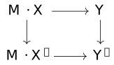
In particular, taking I = \to = \{0 \to 1\} the walking arrow, we obtain a Markov category of deterministic arrows \mathsf {Fun}(\to , \mathcal {C}). We will denote this category simply \mathcal {C}^\to . Again, the objects of this category are the deterministic morphisms of \mathcal {C}, while the morphisms are the commutative squares with not-necessarily-deterministic sides
When we speak of a stochastic map in a Markov category, we always mean a map which is not necessarily deterministic---that is, a general map of \mathcal {C}.
Given a map p: P \to X \otimes Y into a tensor product, the composites with the projections P \to X, P \to Y are called the marginals. Given two maps f: P \to X, g: P \to Y, we refer to any map P \to X \otimes Y with those marginals as a pairing of the two. Note that there is always a canonical pairing given by (f \otimes g) \mathrm {copy}_P. We write \langle f,g \rangle : P \to X \otimes Y for this canonical pairing. For deterministic maps this is just the usual pairing using the universal property of the product. (We mostly use this in cases where one map is deterministic, so that the pairing is unique assuming positivity). When p = \langle \pi _Xp, \pi _Yp \rangle , we say X \bot Y \mid P, and say the two coordinates are independent given P (or just independent).
Recall that the codomain functor \mathcal {C}^\to \to \mathcal {C} is a fibration if and only if \mathcal {C} admits pullbacks. Since Markov categories have terminal objects but not, in general, products, they clearly cannot be expected to have pullbacks.
However, if \mathcal {C} is positive (Reference [fritz-synthetic-markov-cats], def. 11.22---but see Proposition [efr-OYB6] below), given f: P \to Xdeterministic, every g: P \to Y has a unique pairing P \to X \otimes Y with f.
Computing pullbacks X \otimes _Z Y in the subcategory \mathcal {C}_\mathrm {det}, we usually have a similar property. This will be the basic idea behind Markov prefibrations.
By the following straightforward proposition, this property of having unique deterministic pairings is in fact equivalent to positivity:
PropositionCharacterization of positivity[efr-OYB6]
Let \mathcal {C} be a Markov category. The following are equivalent:
In \mathcal {C}, if f: P \to X \otimes Y has deterministic marginal P \to X, then X \bot Y \mid P. In other words, anything is independent of a deterministic variable.
Given a deterministic morphism P \to X and any morphism P \to Y, there is a unique P \to X \otimes Y with those marginals.
Clearly 1 and 2 are equivalent, since independence just means f is the independent pairing of the marginals---if it is uniquely determined by its marginals, it must be equal to the independent pairing, and conversely if it is necessarily independent, it is determined by its marginals. Now let us show this is equivalent to positivity.
First suppose \mathcal {C} has unique pairings in this sense. Let f,g be as in the definition of positivity. Then the two maps X \to Y \otimes Z indicated are pairings of gf and f, and since gf is deterministic, they are identical by hypothesis.
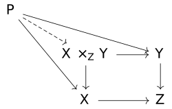
Let \mathcal {C} be a Markov category. We say \mathcal {C} is pullback-positive if \mathcal {C}_\mathrm {det} admits pullbacks and, given a diagram of this form where P \to X is deterministic, there is a unique map P \to X \times _Z Y making the squares commute.
Note that a pullback-positive category is in particular positive by taking Z = I.
The pullbacks appearing in Definition [efr-T3HM] are of course pullbacks in \mathcal {C}_\mathrm {det}, not \mathcal {C}, analogously to how X \otimes Y is a product in \mathcal {C}_\mathrm {det}, not \mathcal {C}. We will still use the notation X \times _Z Y for these pullbacks, which should not lead to any confusion. We may occasionally write X \times Y instead of X \otimes Y, if we are carrying out a construction which primarily involves \mathcal {C}_\mathrm {det}. Since essentially no Markov categories have Cartesian products (except when the tensor product is Cartesian), this should also not lead to any ambiguity.
Suppose any category \mathcal {C}' admits products and intersections---that is, pullbacks U \times _X V whenever U,V are subobjects of X. Then it admits all finite limits.
Suppose \mathcal {C}_\mathrm {det} admits and \mathcal {C}_\mathrm {det} \to \mathcal {C} preserves pullbacks along monomorphisms. Suppose further \mathcal {C} is positive. Then it is pullback-positive.
To see the first point, let f: X \to Z, g: Y \to Z be arbitrary maps. Note that X \times _Z Y = (X \times Y) \times _{X \times Y \times Z \times Z} X \times Y \times Z, where the horizontal map is given by (x,y) \mapsto (x,y,f(x),g(y)), and the top by (x,y,z) \mapsto (x,y,z,z)---in the sense that the universal property of this intersection is exactly the universal property of the given pullback.
Now suppose \mathcal {C}_\mathrm {det} \to \mathcal {C} preserves this intersection, and \mathcal {C} is positive. (Note that it doesn't follow that the inclusion preserves the pullback X \times _Z Y, because it doesn't preserve the products). This amounts to the claim that a map P \to X \otimes Y lifts to the pullback if and only if the composite P \to X \otimes Y \otimes Z \otimes Z lifts over the map 1_X \otimes 1_Y \otimes \mathrm {copy}_Z (note that the pullback of a monomorphism is a monomorphism).
This implies in particular such a lift is always unique. Since if \mathcal {C} is positive, given P \to X, P \to Y, if the latter is deterministic there is a unique pairing P \to X \otimes Y, this implies there is at most one map P \to X \times _Z Y pairing the two. On the other hand, since the composite P \to Y \to Z is deterministic and equal to the composite P \to X \to Z, they are both deterministic, and hence the pairing P \to Z \otimes Z factors over the diagonal. Applying positivity again, to the tensor product (X \otimes Y) \otimes (Z \otimes Z), since the latter component is deterministic, this pairing is independent, and hence the map P \to X \otimes Y \to X \otimes Y \otimes Z \otimes Z does indeed lift, finishing the proof.
The idea here is that a distribution on a subobject X' \subseteq X defined by some condition f(x \in X) \in U \subseteq Y is simply a distribution so that the condition is satisfied with probability 1. This is a natural condition which holds in many Markov categories.
The assumption that \mathcal {C} is pullback-positive will play a key role in the development of the theory of Markov fibrations. Although the theory could possibly be developed without assuming the base category has deterministic pullbacks, positivity seems to be an essential part.
If \mathcal {C} is representable and positive, \mathcal {C}_\mathrm {det} has limits, and the monad P preserves intersections, then \mathcal {C} is pullback-positive.
This is clear, since if the monad P preserves a given limit, so does the inclusion into the Kleisli category (for completely abstract reasons), hence by Lemma [efr-0YP1] we are done.
We will need the notion of support in a Markov category, introduced in Reference [markov-supports], for certain examples, so we briefly record the definition and a few of its properties here.
Let p: X \to Y, q: A \to Y be two morphisms in a Markov category. We say q is absolutely continuous with respect to p and write q << p if, whenever two maps Y \to Z are p-almost surely equal, they are also q-almost surely equal.
Let p: X \to Y be a morphism in a Markov category. The support of p, if it exists, is an object which represents the functor \mathcal {C}(-,Y)_{<<p} of morphisms into Y which are absolutely continuous with respect to p.
The support of p: X \to A is equipped with a canonical deterministic monomorphism S_p \hookrightarrow A, so that a map into A is absolutely continuous with respect to p if and only if it factors over the support.
Two maps A \otimes W \to B are p-almost surely equal if and only if they are strictly equal on the support.
A (strict) double category is a category internal to the category \mathsf {Cat} of categories.
Concretely, it consists of:
A set of objects \operatorname {\mathbf {ob}} \mathbb {C}
A collection of vertical morphisms forming a category \mathbb {C}_v with \operatorname {\mathbf {ob}} \mathbb {C}_v = \operatorname {\mathbf {ob}} \mathbb {C}
A collection of horizontal morphisms forming a category \mathbb {C}_h with \operatorname {\mathbf {ob}} \mathbb {C}_h = \operatorname {\mathbf {ob}} \mathbb {C}
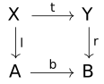
An a collection of squares. Each square has a left and right boundary given by vertical morphisms l,r, and top and bottom boundary given by horizontal morphisms t,b so that \operatorname {\mathrm {dom}} t = \operatorname {\mathrm {dom}} l, \operatorname {\mathrm {cod}} t = \operatorname {\mathrm {dom}} r and so on:
The squares compose horizontally and vertically in the obvious way, each of which form a category (in particular, there are identity squares for each vertical and horizontal map).
A double functor is a mapping on objects, vertical and horizontal morphisms, and squares, which preserves all the identities and composition.
There is also a notion of pseudo double category, which weakens the horizontal composition to only be associative and unital up to a coherent system of squares. We will not go into the details here, see § [efr-000D] for more on this.
There is a pseudo double category \mathsf {\mathbb Cat} where the objects are categories, the vertical maps are functors, the horizontal maps are profunctors (functors \mathcal {C} \times \mathcal {D}^\mathrm {op} \to \mathsf {Set}, sometimes called bimodules), and the squares are natural transformations.
For any category with pullbacks \mathcal {C}, there is a pseudo double category \mathsf {\mathbb Span}(\mathcal {C}) with \mathcal {C} as the vertical category, spans as the horizontal morphisms, and commutative diagrams as the squares.
There is a double category \mathsf {\mathbb Rel} of sets, functions, and relations.
For any Markov category \mathcal {C}, there is a double category with \mathbb {C}_v = \mathcal {C}_\mathrm {det} and \mathbb {C}_h = \mathcal {C}.
For any category at all, there is a double category \operatorname {Sq}(\mathcal {C}) with \operatorname {Sq}(\mathcal {C})_v = \operatorname {Sq}(\mathcal {C})_h = \mathcal {C} and commutative squares as the pullback squares.
A double category is thin if, for each compatible square of vertical and horizontal morphisms, there is at most one square filling it. In other words, such a square either commutes or doesn't.
Sometimes the two classes of morphism are instead called loose and tight, especially in cases where the composition of the loose class is not associative, or if the loose class is a superset of the tight class.
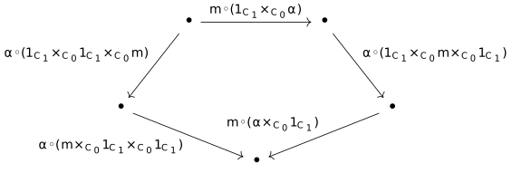
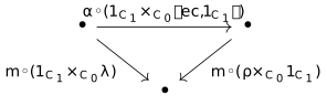
Although the explicit description above is probably the best way to think about the data of a double category, on a technical level it is often useful to think in terms of internal categories. An internal category in a category \mathcal {C} is a pair of objects C_0, C_1, maps d,c: C_1 \to C_0, i: C_0 \to C_1 (the domain, codomain and identity), and a map m: C_1 \times _{C_0} C_1 \to C_1 (the multiplication), satisfying the usual laws of a category. A double category in the above sense is then an internal category in the category of categories.
In the terms of Definition [efr-RXP4], C_0 is \mathbb {C}_v, and C_1 is the category whose objects are horizontal arrows, and whose morphisms are squares (composed vertically). Obviously, we could just as easily have oriented things horizontally, but this is the convention usually adopted.
Given a double category \mathbb {C}, there is another double category \mathbb {C}^T called the transpose of \mathbb {C}, which has the same objects but exchanges the horizontal and vertical morphisms. In many cases it is not clear which of \mathbb {C} and \mathbb {C}^T is the "correct" one to work with, and we may have to pass back and forth between them. We try to stick to the convention that the horizontal morphisms are the "loose" ones. To avoid confusion, we will also simply specify the classes of morphisms directly, speaking for example of "the lenses" or "the charts" when working with the double category \mathsf {\mathbb Arena}(\mathcal {A}) (Definition [efr-0025]).
The concept of double category goes back to Reference [ehresmann-dblcats]. See Reference [johnson-yau-2dim-categories], section 12.3 for a textbook treatment. They have been widely used in applied category theory. An early application is in Reference [baez-courser-structured-cospans], which constructed a "structured" version of the double category of cospans. Here the philosophy is that the horizontal morphisms are the "systems" (in a general sense) which are being wired together by horizontal composition, while the vertical morphisms (and squares) are "structure-preserving maps between systems". This is similar to the our double category of "bisystems" (§ [efr-MWCE]). Recent work by Lambert and Patterson Reference [patterson-lambert-dbltheory] applies double categories to categorical algebra, with many applications to systems modeling, see Reference [catcolab-introducing] (as well as to classical category theory). In the next section we'll see their application to categorical systems theory, and later see them applied to parametrized morphisms.
A theory of dynamical systems is an indexed category \mathcal {A}: \mathcal {C}^\mathrm {op} \to \mathsf {Cat} equipped with a section of its Grothendieck construction T: \mathcal {C} \to \int \mathcal {A}.
It is called monoidal if \mathcal {C} is a monoidal category, and \mathcal {A} is a lax monoidal functor. It is further called symmetric monoidal if \mathcal {C} is a symmetric monoidal category and \mathcal {A} is a symmetric lax monoidal functor. Note that this is equivalent to requiring \int \mathcal {A} \to \mathcal {C} to be a (symmetric) monoidal fibration in the sense of Reference [shulman-monfibs] (see also Reference [moeller-vasilakopoulou]).
Let \mathcal {A}: \mathcal {C}^\mathrm {op} \to \mathsf {Cat} be an indexed category. A chart is simply a morphism in the Grothendieck construction \int \mathcal {A}. A lens is a morphism in the fiberwise opposite \int \mathcal {A}(-)^\mathrm {op}.
Given an indexed category \mathcal {A}: \mathcal {C}^\mathrm {op} \to \mathsf {Cat}, the double category \mathsf {\mathbb Arena} of arenas has
Objects the objects of \int \mathcal {A}---note that these are the same as the objects of \int \mathcal {A}(-)^\mathrm {op}
Vertical morphisms the lenses
Horizontal morphisms the charts
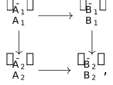
The double category is thin. Given a square of this form
we can first project it to a square in \mathcal {C}. If this commutes, we can pull the lenses and charts back to a square in \mathcal {A}(A_1). The above square of lenses and charts will be said to commute if both of these squares commute.
We will write arenas either as {\bar {A} \in \mathcal {A}(A) \choose A \in \mathcal {C}}, or, for brevity when there is no need to discuss the two levels separately, simply with a symbol A. We will also write both {\bar {TS} \choose S} and TS as the situation calls for---there should be no confusion resulting from this.
DefinitionDynamical system with interface A[efr-0028]
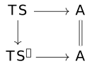
Let A be an arena. A dynamical system with interface A is an object S \in \mathcal {C} and a lens TS \leftrightarrows A. A morphism of systems is a map S \to S' so that this square commutes in \mathsf {\mathbb Arena}:
The category of systems with interface A is denoted \mathsf {Sys}(A)
Given a lens A \leftrightarrows A', postcomposition gives a functor \mathsf {Sys}(A) \to \mathsf {Sys}(A').
Given a chart A \rightrightarrows A', there is a profunctor\mathsf {Sys}(A) \nrightarrow \mathsf {Sys}(A'),
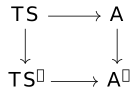
where the set over TS \leftrightarrows A and TS' \leftrightarrows A' is the set of maps S \to S' so that this square commutes:
This defines a double functor \mathsf {Sys}: \mathsf {\mathbb Arena} \to \mathsf {\mathbb Cat}.
The fibration \int \mathcal {A} \to \mathcal {C} encodes what sort of information can be "indexed over a space", while the section T: \mathcal {C} \to \int \mathcal {A} tells us what sort of information (such as a next step, or a gradient vector) must be produced to give a dynamical system. In this respect, the theory is very similar to the coalgebraic approach to dynamical systems, or systems that "do something", and indeed we have the following:
Let F: \mathsf {Set} \to \mathsf {Set} be a functor.
Then there is a dynamical systems theory where \mathcal {C} = \mathsf {Set}, \mathcal {A} is constant at \mathsf {Set},
and T(X) = (X,F(X)). It is easy to see that the category of closed dynamical systems in this theory is equivalently the category of F-coalgebras.
Of course, coalgebras can already encode systems with input and output---the point of the CST framework is to separate out the input and output of systems so that they can be acted on in a compositional manner.
ExampleThe theory of discrete dynamical systems[efr-002F]
There is a theory of dynamical systems with category of spaces \mathcal {C} = \mathsf {Set}, category of bundles \mathcal {A}(X) = \mathsf {Set}_{/X} (with pullbacks for reindexing), and tangent bundle TX = X \times X \xrightarrow {\pi _0} X.
We call this the theory of discrete dynamical systems. (In the sense that they are both discrete-time and discrete-space).
In another direction, we have the following comparison result:
The category of lenses \int \mathcal {A}(-)^\mathrm {op} is equivalently the category of polynomial functors and natural transformations between them.
Using this equivalence, the category of dynamical systems with interface p is exactly the category of p-coalgebras and homomorphisms
The first part here (which works, suitably formulated, for any locally Cartesian closed category), is a classical part of the theory of polynomial functors, see eg Reference [kock-poly-classical]. The second part is due to Spivak, see Reference [spivak-poly-abundant]. There is an extensive body of work on the description of interacting (discrete, deterministic) dynamical systems in terms of polynomial functors, see e.g. also Reference [shapiro-spivak-dynamic-operads].
ExampleThe theory of stochastic discrete dynamical systems[efr-GXJ0]
There is a systems theory where \mathcal {C} = \mathsf {Set}, \mathcal {A}(X) = Kl(\Delta )^X (with the evident reindexing maps) and T(X) = X \times X.
In this theory, a closed dynamical system is a set equipped with a map X \to \Delta (X). An open dynamical system has stochastic update function, but output which depends deterministically on the current system state.
In fact this example works for any monad on the category of sets.
ExampleThe theory of smooth dynamical systems[efr-KZEM]
There is a dynamical systems theory where \mathcal {C} = \mathsf {SmMfd} is the category of smooth manifolds, \mathcal {A}_X is the category of fiber bundles over X, with f^*: \mathcal {A}_Y \to \mathcal {A}_X given by pullback along f: X \to Y (note that pullbacks of bundles always exist), and with TX being the tangent bundle of X in the ordinary sense. In this case, closed dynamical systems are manifolds equipped with (smooth) vector fields, which is what is classically thought of as a smooth dynamical system.
Consider the theory of discrete-time, discrete dynamical systems from Example [efr-002F]. Let \xi : TS \leftrightarrows {I \choose O} be a system.
Consider the system c: T\mathbb {N} \leftrightarrows {* \choose \mathbb {N}} given by n \mapsto n in the forwards direction, and (n,*) \mapsto n+1 in the backwards direction. (To be clear, the object denoted {* \choose \mathbb {N}} is the map \mathbb {N} \to \mathbb {N}---it is a singleton in each fiber). Then a morphism of systems c \to \xi consists of the following data:
A function x: \mathbb {N} \to S.
Another function o: \mathbb {N} \to O.
A third function i: \mathbb {N} \to I so that i(n) \in I_{o(n)}.
So that o(n) = \xi (x(n)) and \xi ^\#(x(n),i(n)) = x(n+1)
That is, it is a choice of a sequence x_n of points in the state-space, and a sequence of inputs i_n compatible with the outputs, so that this sequence obeys the dynamics. In other words, it is a trajectory of the system.
Because of this, one views a generic chart map as a generalized trajectory, of a type given by the domain system. As another example, taking the state space to be \{1,2, \dots , n\} with an update map that carries n to 1, one finds a system which classifies n-periodic trajectories. Similarly, in the smooth case, the system (\mathbb {R}, d/dt: \mathbb {R} \to T\mathbb {R}) classifies solutions of a smooth differential equation (those which extend to infinity).
Recent work by Lynch, Myers, Staton, and the author (Reference [lynch-myers-rischel-staton-stoch-clocks]) constructs clock systems for theories of stochastic, discrete-time doctrines, although we will not delve into this here.
Because this thesis is about Markov fibrations, we have chosen to present these ideas in terms of fibrations equipped with sections. Myers' book Reference [myers-cst] actually prefers the presentation in terms of indexed categories. Similarly, we construct a double category of systems which is fibred (in a certain sense) over the double category of arenas. Myers instead displays this as a doubly indexed category\mathsf {\mathbb Arena} \to \mathsf {\mathbb Cat}, which carries lenses to functors and charts to profunctors.
In a recent paper Reference [double-operadic-systems], Myers and Libkind further develop the category theory of what they term double operadic categorical systems theory, which again concerns notions of "composable system" which are described in terms of such doubly indexed category (although for technical reasons, they use the language of right modules in that paper and a somewhat different presentation, the concept is the same.)
Let Kl(\Delta ) denote the Kleisli category of the discrete (countable) distribution monad on \mathsf {Set}. This is a simple setting for working with probability theory---sufficient for many applications. In order to study compositional Bayesian game theory (Reference [hedges-etal-bayesian-games], Reference [towards-cybercat]) one studies the category \mathsf {Optic}(Kl(\Delta )) of optics in Kl(\Delta ). These have the right level of expressivity to talk about players taking random actions, and where payoff depends stochastically on players' decisions.
In \mathsf {Optic}(Kl(\Delta )),{R \choose X} + {R \choose Y} \cong {R \choose X+Y}. Games with this codomain naturally describe the situation of a player who has a binary choice between X or Y. We call coproducts of this form the "good" coproducts---note that also {* \choose *} + {\emptyset \choose *} = {\emptyset \choose 2}, but this is considered somewhat pathological, since it relies on the nonexistence of any morphism {\emptyset \choose X} \to {A \choose Y} when A and X are nonempty.
In order to describe this structure on \mathsf {Optic}(Kl(\Delta )), it would be useful if it had all coproducts. Unfortunately this is not the case. \mathsf {Optic}(\mathsf {Set}) = \mathsf {Lens}(\mathsf {Set}) has a well-known extension with all coproducts, given by the fiberwise opposite of the fibration \mathsf {Fam}(\mathsf {Set}) \to \mathsf {Set} (this is Proposition [efr-VTPS] in the case \mathcal {C} = \mathsf {Set}). Extending this to stochastic maps would be the obvious way of constructing such a category of "dependent optics".
Consider a category Kl(\Delta )^\to defined as follows. Its objects are the objects of \mathsf {Set}^\to ---that is, they are indexed families of sets. A map in Kl(\Delta )^\to is a stochastic map in the base X \to Y \in Kl(\Delta ), and a stochastic map on the total spaces \bar {X} \to \bar {Y} which is compatible with it. Note that if \bar {X} \to X is surjective, the map on the base is fully determined by the map on the fibers, which must merely satisfy the condition that the distribution of the indexing point in Y depends only on the indexing point in X, not the specific point in the fiber \bar {X}_x.
We claim Kl(\Delta )^\to is a reasonable notion of "stochastic charts". Recall that by "chart" we mean something like "lenses where both maps go forward". If stochastic lenses are supposed to include optics as the full subcategory spanned by the "non-dependent" objects, then the charts should include "co-optics"---that is, maps between X' \otimes X \to X and Y' \otimes Y \to Y should be given by the coend \int ^M \operatorname {\mathrm {Hom}}(X, M \otimes Y) \times \operatorname {\mathrm {Hom}}(X' \otimes M, Y')
And in fact this is the case: Clearly there is a map from this coend to maps in Kl(\Delta )^\to . By taking M = X \otimes Y and conditioning on Y, we see this is surjective. Finally, by restricting to the support of the forwards part inside X \otimes Y, we obtain a representative for each element of the coend which is uniquely determined by X \to Y and X' \times X \to Y' (since the conditional is well-defined on the support).
Note: This relies both on the fact that Kl(\Delta ) has conditionals, and on the existence of supports. We've previously seen these defined in abstract Markov categories (Definition [efr-AB57])--supports in Kl(\Delta ) of a morphism p: A \to B are simply given by those b so that p(b | a) > 0. Note that the existence of both conditionals and supports is a very strong assumption---the only categories we are aware of with both properties are those whose probability distributions have a discrete character, like Kl(\Delta ) and \mathsf {FinStoch}. Neither will be essential to the theory, but both will play a role in certain theorems---we will see more of this later.
The goal of the theory of Markov fibrations is to give a notion of "fiberwise opposite" which can be applied to the codomain functor Kl(\Delta )^\to \to Kl(\Delta ) to give a reasonable notion of "stochastic lenses". In particular, we should recover the usual category of optics in the previous case.
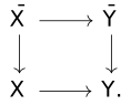
It is clear that the codomain functor is not a (Grothendieck) fibration, since this would require Kl(\Delta ) to have pullbacks, which can only hold for a Cartesian Markov category. However, we can do some things. Namely, given a Cartesian (pullback) square in \mathsf {Set}
and a map {\bar {X} \choose X} \to {\bar {B} \choose B} where the base map X \to B is deterministic, for each deterministic factorizing map X \to A there is a unique lift \bar {X} \to \bar {A}. In other words, the pullback over \mathsf {Set} \hookrightarrow Kl(\Delta ) is a fibration---in fact, it is simply the family fibration \mathsf {Fam}(\mathsf {Kl}(\Delta )).
Furthermore, if \bar {X} \to \bar {B} is itself deterministic, there is such a unique lift even without assuming that the factorization X \to A is deterministic.
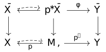
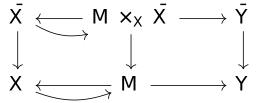
Moreover, we can factor any map in Kl(\Delta )^\to as such an induced map followed by a map over a deterministic base, as follows:
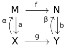
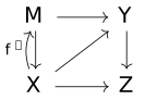
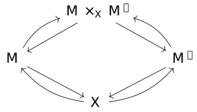
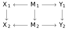
This gives us a hope that we can, in some way, control the category Kl(\Delta )^\to using the pullback over \mathsf {Set}, which is a fibration, and some information somehow given by these extra maps. Note also that the diagram above is equivalent to giving: a span X \leftarrow M \to Y and a section X \to M, which all lives in the base, and a map p^*\bar {X} \to p^{'*}\bar {Y} in the fiber over M. Thus it would seem to be very amenable to fiberwise dualization.
Analogous to our argument above that "co-optics" are equivalent to maps in Kl(\Delta )^\to , we can do the following:
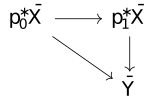
Suppose given two tuples (M_0,p_0,p_0',s_0,\phi _0), (M_1,p_1,p_1',s_1,\phi _1) as above. Suppose there exists a map f: M_0 \to M_1 over X,Y, so that f s_0 = s_1.
Then there is a canonical map p_0^*\bar {X} \to p_1^*\bar {X} over f, because pullbacks commute. If the triangle
moreover commutes, then these two triples represent the same map in Kl(\Delta )^\to
These equivalence relations correspond to "sliding" for deterministic morphisms M \to M'. Note that the condition here can be checked just on the fibration Kl(\Delta )^\to \times _{Kl(\Delta )} \mathsf {Set} \to \mathsf {Set}.
To obtain the full set of sliding equations, we will need to use stochastic maps M \to M', and thus leave that fibration behind. However, we are tantalizingly close to realizing Kl(\Delta )^\to as being presented by some sort of additional structure on the fibration \mathsf {Fam}(\mathsf {Kl}(\Delta )). (For a general monad T acting on C, the category \mathsf {Optic}_{\mathcal {C}}(Kl(T),Kl(T)), of effectful optics up to sliding of pure morphisms, was studied by Riley in Reference [riley-optics], section 4.9, and by Hedges in Reference [hedges-blog-optics-effect])
In this chapter we will indeed provide such a structure, and analyze it. In § [efr-2IMZ], we'll axiomatise the lifting property of Kl(\Delta )^\to discussed above into a property we call a Markov prefibration (Definition [efr-0019]). In § [efr-GO6R], we exhibit a free Markov prefibration associated to a fibration---its morphisms are precisely spans of the form seen above. Naturally, given a prefibration \mathcal {D} \to \mathcal {C}, its underlying fibration on \mathcal {C}_\mathrm {det} becomes an algebra for the monad of this adjunction. In § [efr-U4RA], we characterize the class of prefibrations which are presented by their underlying algebra in this way---these are the Markov fibrations (Definition [efr-HVUT]). Since the monad commutes with fiberwise opposites, this yields a notion of fiberwise opposite for Markov fibrations.
Following this, we review a few properties of the theory of Markov fibrations, including the existence of coproducts in the fibration (Proposition [efr-QAV2]), the stability of Markov fibrations under limits (§ [efr-HWAZ]), and induced monoidal structures (§ [efr-LTEL]). Combining these, we can prove:
Markov categories generally do not have pullbacks, for the same reason that they usually don't have products. This issue generally hinders the construction of fibrations, in the ordinary sense, of Markov categories. However, we can go part of the way. The idea of the following definitions is that given a pullback in the deterministic category, say A \times _Y X, a map P \to A \times _Y Xwhere the X-coordinate is deterministic should be uniquely determined by a choice of (deterministic) map P \to X and (stochastic) P \to A such that the square commutes---as we claimed above (and will see below), this holds for the Markov category of discrete probability Kl(\Delta ). The analogous statement for products---that a map P \to A \otimes X with deterministic X-component is uniquely determined by the projections (or marginals) P \to X, P \to A---is a consequence of positivity (see Proposition [efr-OYB6]), and hence holds in most Markov categories of interest.
Let \mathcal {C} be a Markov category, and let p: \mathcal {D} \to \mathcal {C} be a functor into it.
Then we call p a Markov prefibration if the following two conditions hold:
The pullback \mathcal {D} \times _\mathcal {C} \mathcal {C}_\mathrm {det} \to \mathcal {C}_\mathrm {det} is a (Grothendieck) fibration
Given maps f: A \to C, g:B \to C in \mathcal {D}, such that p(f),p(g) are deterministic and f,g are Cartesian for the above fibration, p induces a bijection between maps h: A \to B \in \mathcal {C} such that gh = f, and maps h': p(A) \to p(B) so that p(g)h' = p(f). Note that when restricted to those maps where p(h) is deterministic, this being a bijection is the defining property of g being Cartesian (for any f, not necessarily a Cartesian one).
Given a Markov prefibration \mathcal {D}, we write \mathcal {D}|_\mathrm {det} for \mathcal {D} \times _\mathcal {C} \mathcal {C}_\mathrm {det}. We will refer to this as the deterministic part of \mathcal {D}---note that this does have the potential for confusion, as when \mathcal {D} is itself a Markov category, this is not necessarily the same as the deterministic subcategory of \mathcal {D}. When f \in \mathcal {D} lies inside \mathcal {D}|_\mathrm {det}, and is Cartesian for that fibration, we will simply refer to it as a Cartesian map in \mathcal {D} (there are no other types of Cartesian maps, so this should not lead to confusion). A morphism of Markov prefibrations is a functor \mathcal {D} \to \mathcal {D}' over \mathcal {C} which preserves Cartesian maps. The category of Markov prefibrations over \mathcal {C} thus defined is denoted \mathsf {MarkPreFib}(\mathcal {C}). Taking the deterministic part defines a functor (-)|_\mathrm {det}: \mathsf {MarkPreFib}(\mathcal {C}) \to \mathsf {Fib}(\mathcal {C}_\mathrm {det}).
Since we will shortly be working with a number of functors between categories whose objects are themselves categories with some structure, it may be thought that we should give some consideration to the strictness of our constructions---for example, we will shortly construct a left adjoint to (-)|_\mathrm {det}: \mathsf {MarkPreFib}(\mathcal {C}_\mathrm {det}) \to \mathsf {Fib}(\mathcal {C}), and it may well be asked how strict this adjoint is, whether we need to consider the definition of pseudomonad when we get so far, et cetera.
However, we can largely avoid this issue. The key observation is that none of our functors will alter the objects of the underlying category (since \mathcal {C}_\mathrm {det} \to \mathcal {C} is identity on objects,). Hence, all the natural transformations that we would ordinarily ask to be equivalences of categories will instead be isomorphisms, and we can largely ignore considerations of higher category theory---similarly, all our functors will be strictly functorial. As a simple example of this, observe that the pullback functor (-)|_\mathrm {det} is automatically strict---it simply consists in restriction to a subset of the morphisms in \mathcal {D} (which is automatically closed under composition), and thus clearly preserves composition strictly.
In a Markov prefibration p: \mathcal {D} \to \mathcal {C} (as previously noted), a morphism f: \bar {X} \to \bar {Y} in \mathcal {D} is called Cartesian if p(f) is deterministic and f is Cartesian in the fibration \mathcal {D}|_\mathrm {det} \to \mathcal {C}_\mathrm {det}. It is called vertical if p(f) is an identity. It is called a stochastic-Cartesian if there exists a Cartesian map r: \bar {Y} \to \bar {X} so that rf = 1_{\bar {X}} (recall that in this case f is uniquely determined by r and p(f)). Note that if f is stochastic-Cartesian and p(f) is deterministic, then f is Cartesian.
The introduction to this chapter contains the argument that Kl(\Delta ) is a Markov prefibration. This is a key motivating example.
ExampleMarkov prefibrations over Cartesian base[efr-CJTH]
Let \mathcal {C} be a Markov category which is Cartesian (that is, one where all morphisms are deterministic). Then a Markov prefibration over \mathcal {C} is simply a Grothendieck fibration.
Let \mathcal {C} be a Markov category. Then \mathcal {C}^\to \to \mathcal {C} is a Markov prefibration with Cartesian maps given by pullback squares, if and only if \mathcal {C} is pullback-positive.
Assume first \mathcal {C} is pullback-positive. It is clear that computing pullbacks in \mathcal {C}_\mathrm {det} gives the required Cartesian lifts---pullback positivity is precisely the claim that lifts exist uniquely in the definition of a Cartesian morphism (since the map to the base leg of the pullback is always deterministic in this case). Since Cartesian lifts can be taken to be deterministic (we have just constructed deterministic Cartesian lifts, and such lifts are unique up to unique isomorphism), the second condition also follows from this assumption, simply taking the other leg to be deterministic.
Conversely, suppose \mathcal {C}^\to \to \mathcal {C} is a Markov prefibration and suppose the Cartesian maps are given by the deterministic pullback squares.
Let Y \to Z be an object of \mathcal {C}^\to and let X \to Z be a deterministic map, and form the pullback X \times _Z Y, which is Cartesian. Let P \to X be deterministic and let P \to Y be any map. Expanding the latter into a map from the object P \to P to Y \to Z, the Cartesian property of the square implies there is a unique pairing P \to X \times _Z Y
In a general Markov category, not every isomorphism is necessarily deterministic. This means that, in general, fibres over isomorphic objects in a Markov prefibration are not necessarily isomorphic or even equivalent as categories. This seemingly immoral situation is, in fact, in accordance with other results indicating that deterministic isomorphism is really the proper notion of identification in a Markov category. See eg Reference [rischel-fritz-infinite-products], Section 4, for further discussion of this point. (Since the basic idea of a Markov category involves objects equipped with some structure which is not preserved by all the morphisms, it is not so paradoxical that an isomorphism in this situation should be insufficient to render two objects identical).
Under very weak assumptions on the Markov category \mathcal {C}, such as positivity, all isomorphisms are deterministic. This implies that all Markov prefibrations over \mathcal {C} are isofibrations, and thus rules out any sort of behavior like the above. As noted, we are only concerned with positive Markov categories.
Relatedly, in the proof of Proposition [efr-0044], a careless prover may have erroneously concluded after the first step that all Cartesian lifts are deterministic---but since Cartesian lifts are characterized only up to isomorphism, not necessarily deterministic isomorphism, this does not automatically follow. (But of course replacing a nondeterministic lift with an isomorphic deterministic one in this situation cannot alter the unique existence of the factorization, so it does not matter).
Let p: \mathcal {D} \to \mathcal {C} be a Markov prefibration, let \mathcal {C}' \subseteq \mathcal {C}, \mathcal {D}' \subseteq \mathcal {D} be full subcategories so that p(\mathcal {D}') is contained in \mathcal {C}',
and suppose \mathcal {C}' is a monoidal subcategory (which is then automatically a sub-Markov category). Suppose finally \mathcal {D}' is stable under pullback along deterministic morphisms in \mathcal {C}'. Then \mathcal {D}' \to \mathcal {C}' is again a Markov prefibration.
By assumption, given Y \in \mathcal {D}' and f: X \to p(Y) \in \mathcal {C}', the Cartesian lift X' \to Y is again in \mathcal {D}'. The fullness of the subcategory inclusions suffices to prove the existence and uniqueness of the required lifts so that this is still Cartesian after restricting. For the same reason, since we have just observed that the Cartesian lifts are the same as in \mathcal {D} \to \mathcal {C}, the second part of the definition also holds.
Example\mathsf {Stoch}^\to as Markov prefibration[efr-NC7D]
Recall that the deterministic maps in \mathsf {Stoch} are those kernels valued in \{0,1\}-valued measures. (And that these are not the same thing as the measurable maps).
Given a pair f:X \to Z, g: Y \to Z of such maps, we claim that the subset of X \times Y given by those points where f(x) = g(y) as measures on Z, equipped with the subset \sigma -algebra and its inclusions into X and Y, is a pullback in \mathsf {Stoch}_\mathrm {det}.
To see this, observe that \mathsf {Stoch}_\mathrm {det} is the Kleisli category for the submonad G_{0,1} of the Giry monad which takes a space to the subspace of 0,1-valued probability measures on it. Note that by the general theory of Markov categories this has products given by the products in \mathsf {Meas}. It hence suffices to prove that the pullback of f \times g: X \times Y \to Z \times Z along the diagonal Z \to Z \times Z exists---if it does, it has the universal property of the product X \times _Y Z.
To see that it does (and that it's given by the space described above), note that the diagonal is a split monomorphism, so it suffices to show that h: P \to X \times Y \in \mathsf {Stoch}_\mathrm {det} factors over X \times _Y Z if and only if the composite to Z \times Z lifts over the diagonal.
Now this lift over Z exists if and only if the probability of the diagonal \operatorname {im}(Z) \subseteq Z \times Z under the composite is 1. By definition, it is
\int f(\operatorname {im}(Z) \mid x) g(\operatorname {im}(Z) \mid y) h(dx,y \mid p)
Since the function being integrated is an indicator, this is simply the measure of the set \{(x,y) : \mathbb {P}(\operatorname {im}(Z) \mid x,y) = 1\}.
If the probability of the diagonal is one, clearly the two marginals agree. Conversely, since \mathsf {Stoch}_\mathrm {det} is Cartesian, it must be the case that if the marginals agree the probability of the diagonal is 1. Therefore this is equal to the subset X \times _Z Y \subseteq X \times Y described at the start. But for this to have measure 1 for all p \in P is equivalent to the desired lifting property. This finishes the argument.
Moreover, this argument relied only on the 0,1-valuedness of the maps f,g, not h: P \to X \times Y or its marginals. Hence this also proves that the pullback along the diagonal is preserved by the inclusion \mathsf {Stoch}_\mathrm {det} \to \mathsf {Stoch}.
Since \mathsf {Stoch} is known to be positive, this implies \mathsf {Stoch}^\to \to \mathsf {Stoch} is a Markov prefibration.
We wish to apply Proposition [efr-0042]. The only thing to check is that standard Borel spaces are stable under pullbacks in \mathsf {Meas}.
But standard Borel spaces are known to be stable under products and measurable subsets, and this is enough (see eg. Reference [srivastava-borelsets] propositions 3.1.23 and 3.3.15)
The functor \mathsf {Optic}(\mathsf {BorelStoch}) \to \mathsf {BorelStoch} is not a Markov prefibration, although its pullback over \mathsf {BorelStoch}_\mathrm {det} is a Grothendieck fibration.
To see this, first consider the deterministic pullback. An optic \binom {A}{X} \to \binom {B}{Y} with deterministic base can be identified with a map X \otimes B \to A (and the base deterministic map X \to Y). To see this, first observe that the subset of \mathsf {BorelStoch}(X, Y \otimes M) with the marginal X \to Y deterministic is in bijection with \mathsf {BorelStoch}_\mathrm {det}(X,Y) \times \mathsf {BorelStoch}(X,M), since \mathsf {BorelStoch} is positive. Hence we can calculate
\int ^M \mathsf {BorelStoch}_\mathrm {det}(X,Y) \times \mathsf {BorelStoch}(X,M) \times \mathsf {BorelStoch}(M \otimes B, A) \cong \mathsf {BorelStoch}_\mathrm {det}(X,Y) \times \mathsf {BorelStoch}(X \times B, A),
using the ninja yoneda lemma as in Proposition [efr-M19V].
Hence this part is a fibration with the fiber over X being the coKleisli category of the X \times - monad, and the pullback functors given by reindexing these parametrized maps. The Cartesian lift of a map X \to Y at \binom {B}{Y} is given by the optic \binom {B}{X} \to \binom {B}{Y} with unit residual and identity backwards component.
Now, let g: I \to \mathbb {R} denote the standard Gaussian distribution, let f: \mathbb {R} \otimes \mathbb {R} \to \mathbb {R} be the function given by f(x,y) = 0 if x=y and y otherwise, and consider the two optics \binom {\mathbb {R}}{*} \to \binom {\mathbb {R}}{\mathbb {R}} given by (I, g: I \to \mathbb {R}, 1_\mathbb {R}: \mathbb {R} \to \mathbb {R}), (\mathbb {R}, \mathrm {copy}_\mathbb {R} g : I \to \mathbb {R} \otimes \mathbb {R}, f: \mathbb {R} \otimes \mathbb {R} \to \mathbb {R}) (where we recall that the first argument is the residual). They cannot be equal, as postcomposition with the optic \binom {\mathbb {R}}{\mathbb {R}} \to \binom {*}{*} given by the identity \mathbb {R} \to \mathbb {R} yields, for the former, the standard Gaussian g: I \to \mathbb {R}, and for the latter, the constant zero map. But postcomposition with the projection \binom {\mathbb {R}}{\mathbb {R}} \to \binom {\mathbb {R}}{*} does give the same optic (the identity), because, for every fixed y \in \mathbb {R}, when x is normally distributed, f(x,y) = y with probability one. Hence the unique lifting of Cartesian maps over Cartesian maps cannot hold.
This counterexample indicates that, although \mathsf {BorelStoch}^\to is a Markov prefibration, we can not expect a dual version of this prefibration---in fact, since over deterministic maps \mathsf {Optic}(\mathsf {BorelStoch})is the fiberwise dual of (the restriction to trivially-indexed objects of) \mathsf {BorelStoch}^\to , this example shows that there is no Markov prefibration whose deterministic part is the fiberwise dual of \mathsf {BorelStoch}. Moreover, as the example indicates, this is not a mere technical issue, but an unavoidable fact about optics in general measurable spaces---even up to behavioral equivalence, they simply don't satisfy the conditions of being a Markov prefibration. (But see Theorem [efr-K6NM])
As above, we see that the deterministic part is a fibration, so take X \to Y \leftarrow Z deterministic maps, and let \binom {A}{X} \to \binom {A}{Z} be an optic so that the induced triangle with the two Cartesian lifts to \binom {A}{Y} commutes. Let the two parts be f: X \to M \otimes Y, g: M \otimes A \to A. The implication is that X \to M \otimes Y \to M -almost surely, g is equal to the projection to A (and X \to M \otimes Y \to Y renders the triangle in \mathcal {C} commutative). Note that f factors over the support of this map, hence we can assume the marginal X \to M has full support. Hence up to sliding equivalence, g is strictly equal to the projection. This implies the lift is uniquely determined as desired.
The existence of supports rules out the pathological behaviour. Essentially, in the presence of supports, we can sensibly reason about "the points of measure zero" and exclude them from consideration---and Proposition [efr-8MYE] implies that the independent pairing of two measures always have the least "points of measure zero", and so that what can be proven equivalent under the assumption of independence will always be equivalent. By contrast, the map f: \mathbb {R} \times \mathbb {R} \to \mathbb {R} from Example [efr-8B5X] satisfies f(x,y) = y for almost all x when x is normally distributed, for all y, but this does not imply that for all measures on x,y with this marginal, f(x,y) is distributed as the marginal of y.
One point of view is that the map f is simply pathological, and we should restrict our attention to maps that are continuous in some sense (from the point of view of computer science, one argument for this is that computable maps are necessarily continuous). The category \mathsf {TychStoch} of Tychonoff spaces and weakly continuous kernels does indeed have supports. However, since it lacks conditionals, it is still not ideal from our point of view.
Because every map in Kl(\Delta )^\to factors into arrows which are "induced" from arrows in Kl(\Delta )^\to |_\mathrm {det} and the Markov prefibration property, it may initially be hoped that Kl(\Delta )^\to is in some sense "free" on the data of the fibration Kl(\Delta )^\to |_\mathrm {det} \to \mathsf {Set} and the inclusion \mathsf {Set} \to Kl(\Delta ). If that was true, we may further hope that taking the fiberwise opposite of the fibration and applying the same free generation principle would generate a good notion of stochastic lens.
Unfortunately, this is not the case. We will see that the free prefibration is given by gadgets which look a bit like an indexed version of optics, up to a sliding equivalence for deterministic maps on the residual. This prompts us to look for some extra structure on the fibration \mathcal {D}|_\mathrm {det} \to \mathcal {C}_\mathrm {det} which describes sliding equivalences for stochastic maps on the residual. In the next section, we will see that this is exactly the structure of an Eilenberg-Moore algebra for the free prefibration monad on \mathsf {Fib}(\mathcal {C}_\mathrm {det}).
In this section, we will give a description of the free Markov prefibration on a fibration \mathcal {D}_0 \to \mathcal {C}_{\mathrm {det}} (assuming \mathcal {C} is pullback positive). There is a fairly simple description of the hom-sets, but their composition is a bit tricky, and verifying associativity even more so. Hence we will employ a technical trick: by characterizing the hom-sets as "freely generated" in a certain sense from the hom-sets in \mathcal {D}_0, we can identify them with sets of natural transformations using a Yoneda-type argument, and infer composition and associativity from there.
Let p: \mathcal {D} \to \mathcal {C} be a functor. An indexed copresheaf on \mathcal {D} is a tuple (X \in \mathcal {C}, F: \mathcal {D} \to \mathsf {Set}, \alpha : F(-) \to \mathcal {C}(X,p(-))) consisting of a copresheaf, an object of \mathcal {C}, and a natural transformation \alpha as indicated. We say the indexed copresheaf is overX, and we will abuse the terminology by referring to F itself as an indexed copresheaf, leaving the transformation \alpha implicit (for example, "let F be an indexed copresheaf over X").
We denote the subset \alpha ^{-1}(\{f\}) \subseteq F(\bar {A}), for f: X \to p(\bar {A}) by F(\bar {A})_f.
A map of indexed copresheaves (X,F,\alpha ) \to (Y,G,\beta ) is a natural transformation F \to G and a map Y \to X \in \mathcal {C} so that the obvious square of natural transformations commutes. We denote the category of indexed copresheaves by \mathsf {IcoPSh}(\mathcal {C} / \mathcal {D}). Note that there is an obvious forgetful functor \mathsf {IcoPSh}(\mathcal {D} / \mathcal {C})^\mathrm {op} \to \mathcal {C}
Observe that for each object A \in \mathcal {D}, there is a corepresentable copresheaf (p(A), \mathcal {D}(A,-), p). Maps between these obey the Yoneda lemma, in the sense that they are in bijection with maps between the underlying objects in \mathcal {D}. This defines a fully faithful functor \mathcal {D} \to \mathsf {IcoPSh}(\mathcal {D} / \mathcal {C})^\mathrm {op} over \mathcal {C}.
Of course, there is a dual notion of indexed presheaf, but this will not interest us.
Let p: \mathcal {D} \to \mathcal {C} be any functor and let \mathcal {C}_0 \to \mathcal {C} be an identity-on-objects functor. Write \mathcal {D}_0 = \mathcal {D} \times _\mathcal {C} \mathcal {C}_0 for the pullback. If F: \mathcal {D} \to \mathsf {Set} is a copresheaf indexed over X \in \mathcal {C},
the pullback \bar {A} \mapsto F(\bar {A}) \times _{\mathcal {C}(X,p\bar {A})} \mathcal {C}_0(X,p\bar {A}) is a copresheaf on \mathcal {D}_0 indexed over X again in a unique way. This defines a functor \mathsf {IcoPSh}(\mathcal {D} / \mathcal {C}) \to \mathsf {IcoPSh}(\mathcal {D}_0 / \mathcal {C}_0). Moreover, this functor preserves the corepresentable copresheaves (since \mathcal {C}_0 \to \mathcal {C} is identity on objects, so is \mathcal {D}_0 \to \mathcal {D}, so this statement makes sense).
Let \mathcal {D}_0 \to \mathcal {C}_0 be a functor and let \mathcal {C}_0 \to \mathcal {C} be identity-on-objects and faithful.
Then the pullback of the composite \mathcal {D}_0 \to \mathcal {C} and the inclusion \mathcal {C}_0 \to \mathcal {C} is identical to \mathcal {D}_0.
Therefore, Proposition [efr-FOJT] gives a functor \mathsf {IcoPSh}(\mathcal {D}_0 / \mathcal {C}) \to \mathsf {IcoPSh}(\mathcal {D}_0 / \mathcal {C}_0).
The idea of our construction of the free Markov prefibration is to give a certain monad on \mathsf {IcoPSh}(\mathcal {D}_0 / \mathcal {C}) and consider the Kleisli maps between the representable copresheaves.
At this point, the notion of a deterministic map M \to X equipped with a stochastic (ie not necessarily deterministic) section begins playing a key role. The phrase "stochastic section" will always carry an implicit "of a deterministic map". In most cases the map that the section is a section of will be clear from the context.
Note that, given a stochastic section Y \to M and a deterministic map X \to Y, if \mathcal {C} is pullback-positive, there is a unique lifting of this to a section of the projection Y \times _X M \to Y. We will use this fact several times.
Let \mathcal {C} be a Markov category, and let \mathcal {D}_0 \to \mathcal {C}_\mathrm {det} be a fibration.
Then a stochastic module consists of
An indexed copresheaf F = (A,F,\rho ) \in \mathsf {IcoPSh}(\mathcal {D}_0 / \mathcal {C})
For each \bar {X} \in \mathcal {D}_0, Cartesian morphism \bar {a}: \bar {X}_M \to \bar {X} lying over a: M \to X, and stochastic section \alpha : X \to M, a function \alpha _*: F(\bar {X}) \to F(\bar {X}_M), which acts on the underlying morphisms in \mathcal {C} as composition with \alpha
Satisfying, whenever given a commutative square of Cartesian morphisms:
and stochastic sections \alpha ,\beta lying over a = p(\bar {a}), b = p(\bar {b}), so that we have a digram in \mathcal {C}:
Where the maps except \alpha ,\beta are deterministic, \alpha and \beta are sections of a and b, and both the square of deterministic maps and the square involving \alpha ,\beta commute, the condition that the square
commutes.
And satisfying furthermore the equation, for every two stochastic sections \alpha :X \to M,\beta : M \to N, the equation (\beta \alpha )_* = \beta _*\alpha _* (note that this makes sense because pullbacks compose).
A morphism of stochastic modules is an indexed natural transformation which preserves the operations \alpha _*. The category of stochastic modules is denoted \mathsf {SMod}(\mathcal {D}_0 / \mathcal {C}). There is an apparent forgetful functor \mathsf {SMod}(\mathcal {D}_0 / \mathcal {C}) \to \mathsf {IcoPSh}(\mathcal {D}_0 / \mathcal {C}).
Note that \alpha _* of course depends on f, not just \alpha .
If f: M \to X is a deterministic map, \alpha :X \to M is a stochastic section, and \bar {X}_M, \bar {X}_M' \to \bar {X} are two Cartesian lifts of f to \bar {X} \in \mathcal {D}_X, then applying the commutativity axiom for stochastic modules implies that the triangle
commutes. In what follows, we will simply write f^*\bar {X} for some choice of cartesian lift, and speak of \alpha _* : F(\bar {X}) \to F(f^*\bar {X}). The above shows that this is a harmless abuse---the actions \alpha _* are preserved by the identification of different Cartesian lifts. In particular, we will often make arguments as if pullbacks compose strictly, although in general they only compose up to isomorphism. The above triangle means this is harmless.
The term "stochastic module" is not very good, but this is mostly a nonce definition in any case, so we won't worry too much about it.
Stochastic modules over a given X \in \mathcal {C} can be seen to be monadic over the category of indexed copresheaves over that X. However, the compatibility of these local left adjoints with the structure of the rest of the category is somewhat subtle. However, we do have free stochastic modules on representable indexed copresheaves, as we will soon see.
Let \mathcal {D} \to \mathcal {C} be a Markov prefibration, and let \mathcal {D}_0 = \mathcal {D} \times _\mathcal {C} \mathcal {C}_\mathrm {det}. Then the corepresentable copresheaf \mathcal {D}(\bar {A},-), restricted to \mathcal {D}_0, (but not pulled back---that is, we remember the whole set \mathcal {D}(\bar {A},\bar {X}), even the part over stochastic f, but only the composition with maps in \mathcal {D}_0) is a stochastic module in a canonical way, with \alpha _*: F(\bar {X}) \to F(f^*\bar {X}) given by composition with the unique induced lift of \alpha . Moreover, any morphism of Markov prefibrations \phi : \mathcal {D} \to \mathcal {D}' induces a homomorphism of stochastic modules \mathcal {D}(\bar {A},-) \to \mathcal {D}'(\phi (\bar {A}),-)
Given f: M \to X and a stochastic section \alpha , it's clear that composition with the unique lift \bar {X} \to f^*\bar {X} is a map of the right type, so we just have to verify the equations.
For the first equation (item 3 in the definition of stochastic module), we are comparing two maps F(g^*\bar {X}) \to F(b^*\bar {X}). These are given by composition with two maps, let's call them \\phi, \psi : g^*\bar {X} \to b^*\bar {X}. These two maps are lifts of f\alpha and \beta g, but by assumption these two are equal. Hence by the uniqueness property of Markov prefibrations, \phi = \psi , and we have our equation. The other equation follows in a completely analogous way.
To prove the homomorphism property, note that a morphism of prefibrations preserves Cartesian morphisms, and hence (by uniqueness) must preserve the unique lifts of stochastic sections. Then by functoriality it must preserve composition with these, which finishes the proof.
Let \bar {X} \in \mathcal {D}_0 be an object. Then there is a free stochastic module T\mathcal {D}_0(\bar {X},-) on its representable copresheaf, in the sense that if F is another stochastic module, homomorphisms T\mathcal {D}_0(\bar {X},-) \to F are in bijection with indexed natural transformations \mathcal {D}_0(\bar {X},-) \to F
The free stochastic module on a corepresentable presheaf is given as follows: an element of T\mathcal {D}_0(\bar {X},-)(\bar {Y}) consists of a diagram in \mathcal {C} of the form
(where X = p(\bar {X}), Y = p(\bar {Y}),) where fs = 1_X and f,g are deterministic, plus a map f^*\bar {X} \to \bar {Y} lying over g. This is up to the equivalence relation which, given some other such tuple, identifies them whenever there exists deterministic h: N \to M as in this diagram:
so that the two deterministic triangles commute, hs' = s, and so that the unique Cartesian map f'^*\bar {X} \to f^*\bar {X} over h forms a commutative triangle with the two maps to \bar {Y}. (Note that we do not claim the relation just described is inherently an equivalence relation, rather we form the equivalence relation generated by this). It is clear how a map \bar {Y} \to \bar {Z} acts on this to make it a copresheaf. It is indexed by taking a tuple as above to the composite X \to M \to Y. Given N \to Y with a stochastic section s': Y \to N,, and an element of T\mathcal {D}_0(\bar {X},-)(\bar {Y}), the induced element in T\mathcal {D}_0(\bar {X},-)(s'^*\bar {Y}) is given by forming the pullback M \times _Y N, taking the pullback of the map over g to one lying over the projection M \times _Y N \to N, and composing the section s with the induced lift M \to M \times _Y N
The underlying copresheaf of this respects Cartesian maps in \mathcal {D}_0 \to \mathcal {C}_\mathrm {det}, in the sense that given a Cartesian map \bar {A} \to \bar {B} and an element \phi \in T\mathcal {D}_0(\bar {X},-)(\bar {B}) lying over a deterministic map X \to B, the natural map from lifts \psi \in T\mathcal {D}_0(\bar {X},-)(\bar {A}) to lifts X \to A is a bijection.
First, we have to verify the equations of a stochastic module for T\mathcal {D}_0(\overline {X},-). For the first case, suppose we are given a square
with all but the upwards maps stochastic. Now let \bar {Z} be some object over Z and suppose we are given an element of T\mathcal {D}_0(\bar {X}, \bar {Z}_Y), represented by a span
X \leftarrow M \to Y, a section X \to M and a map \phi : \bar {X}_M \to \bar {Z}_M over M.
Consider then the below diagram:
By definition, the first of the two possible elements of T\mathcal {D}_0(\bar {Z}_W) are given by either forming the pullback M \times _Y N, taking the lift of \alpha to M \to M \times _Y N and composing to get a section X \to M \times _Y N, and pulling back \phi along the projection to get a map \bar {X}_{M \times _Y N} \to \bar {Z}_{M \times _Y N}, then taking the span X \leftarrow M \times _Y N \to W.
The second is given by first composing with the map Y \to Z, then applying the above procedure with the pullback M \times _Z W. The induced map M \times _Y N \to M \times _Z W exhibits the equality of these two under the equivalence relation defining T\mathcal {D}_0(\bar {X},-) (commutativity of the bottom-right square implies that triangle of stochastic sections commutes.)
Given some other stochastic module F over A with a map of indexed copresheaves \mathcal {D}_0(\bar {X},-) \to F, over A \to X, there is at most one extension to a map of stochastic presheaves T\mathcal {D}_0(\bar {X},-) \to F over A \to X---given an element with representative (s:X \to M, X \leftarrow M \to Y, \bar {X}_M \to \bar {Y}_M), it must go to the identity element of F(\bar {X}), acted on by the stochastic section s to produce an element of F(\bar {X}_M), followed by F applied to the map \bar {X}_M \to \bar {Y} over M \to Y.
But it is not hard to see that the equivalence relation imposed by T\mathcal {D}_0(\bar {X},-) is implied by the equations of a stochastic module, and so this map is well-defined, establishing the property.
Secondly, let \bar {A} \to \bar {B} be a Cartesian map over A \to B, and take a commutative triangle
of deterministic maps. Finally take an element of T\mathcal {D}_0(\bar {X},-)(\bar {B}) over the given map X \to B. We must show it has a unique lift to A over the given map X \to A.
Let us take a representative given by a diagram:
First, note that the two maps M \to X \to B and M \to B do not necessarily agree. However, we can remedy this by replacing M by their equalizer---note that as we argued above, this gives an equivalent element of the stochastic module. (By writing their equalizer in \mathcal {C}_\mathrm {det} as the split pullback M \times _{B \times B} B, we can see that the section factors over this, even if \mathcal {C} does not have all equalizers in general). Hence we can assume the triangle formed by adding the dashed arrow commutes.
Since M \to B now factors over X, the lift X \to A gives a lift M \to A. Now by the Cartesian property of \bar {A} \to \bar {B}, there is a unique lift of p^*\bar {X} \to \bar {B} to this map (here we just use the fact that \mathcal {D}_0 is a fibration). This gives the desired lift.
Finally, given two distinct lifts (again, we can assume their maps M \to A factor over X,) clearly any map N \to M witnessing an identity between their composites \bar {X} \to \bar {Y} would likewise exhibit an identity between their lifts (since pullbacks compose). This proves uniqueness, and finishes the proof.
We are now ready to prove the main proposition of this section:
Let \mathcal {C} be a pullback-positive Markov category and let \mathcal {D}_0 \to \mathcal {C}_\mathrm {det} be a fibration. Consider the full subcategory of stochastic modules spanned by the free modules on the corepresentables. Denote the opposite of this category \bar {\mathcal {D}_0}. Clearly there is a commutative diagram
We claim:
\bar {\mathcal {D}_0} \to \mathcal {C} is a Markov prefibration.
There is a bijection \bar {\mathcal {D}_0}(\bar {A},-) \cong T(\mathcal {D}_0(\bar {A},-)). When the left-hand side is equipped with the canonical stochastic module structure, and the right is equipped with the free one, this is moreover a homomorphism (hence isomorphism) of stochastic modules.
\bar {\mathcal {D}_0} \to \mathcal {C} is initial among Markov prefibrations receiving a map from \mathcal {D}_0. In other words, this construction gives a left adjoint to the pullback functor \mathsf {MarkPreFib}(\mathcal {C}) \to \mathsf {Fib}(\mathcal {C}_\mathrm {det})
First observe that, by Lemma [efr-OH7U], the pullback \bar {\mathcal {D}_0}\times _\mathcal {C} \mathcal {C}_\mathrm {det} \to \mathcal {C}_\mathrm {det} is indeed a fibration, with the image of the Cartesian lifts under the functor \mathcal {D}_0 \to \bar {\mathcal {D}_0} being Cartesian again. (This also establishes that \bar {\mathcal {D}_0} really does receive a map of fibrations from \mathcal {D}_0)
Given Cartesian f: \bar {A} \to \bar {B} \leftarrow \bar {C}, and a stochastic lift A \to C (= p\bar {A} \to p\bar {C}), consider the pullback A \times _B C, and the pullback of \bar {A} to it. There is a unique lift of A \to C to a section A \to A \times _B C, and this induces a unique lift \bar {A} \to (f\pi _1)^*\bar {A} using the stochastic module structure. The composite of this with the projection to B is a lift of \bar {A \to \bar {B}} over A \to C, as required by a Markov prefibration.
Analogously to the proof of Lemma [efr-OH7U], given some other lift A \leftarrow N \to C, h: A \to N, h^*\bar {A} \to \bar {C}, the fact this is a factorization implies the existence of some M with maps M \to A, M \to N and a lift A \to M of the section A \to N, so that the induced map between the pullbacks over M and N of \bar {A} makes the triangle into \bar {B} commute. But then since this is a triangle over deterministic bases, this implies the lifted triangle to \bar {C} also commutes, hence this M lifts to another representative of the lift we started with. But then it's not hard to see that this M maps to A \times _B C and exhibits an equation with the previously constructed "canonical" lift.
Hence \bar {\mathcal {D}_0} is a Markov prefibration, and by the above, the induced stochastic module structure on the corepresentable presheaves \bar {\mathcal {D}_0}(\bar {A},-) = T(\mathcal {D}_0(\bar {A},-)) is exactly the one given by T (in other words this equation is not merely a bijection of sets, but an isomorphism of stochastic modules).
Let \phi : \mathcal {D}_0 \to \mathcal {D}' be a functor over \mathcal {C}_\mathrm {det} \to \mathcal {C} into some other Markov prefibration which preserves Cartesian maps. Using the algebra structure on \mathcal {D}'(\phi \bar {B},-), we see there is a unique extension of \phi to \bar {\mathcal {D}_0}(\bar {X},-) which respects the stochastic module structure. By chasing the diagram around it's easy to see that this is functorial, and hence gives a map of Markov prefibrations---conversely, any such map extending \phi must be a stochastic module homomorphism. Thus there is a unique functor, proving initiality.
This characterization of the left adjoint makes it fairly easy to understand the induced monad on \mathsf {Fib}(\mathcal {C}_\mathrm {det}).
We will sometimes refer to the morphisms of \overline {\mathcal {D}_0} as precharts. Taking the fibration \mathcal {C}^\to |_\mathrm {det} \to \mathcal {C}_\mathrm {det} as an example, it is not too hard to see that the precharts between X \otimes A \to X and B \otimes Y \to Y are representatives of co-optics {A \choose X} \rightrightarrows {B \choose Y}. (To see this, note that any prechart is equivalent to one where the apex of the span has the form M \otimes Y and the right leg is the projection to Y. Then the rest of the data is a map X \to M \otimes Y and a map M \otimes B \to A, since the X-coordiante of the latter map is determined by the span).
In fact their equivalence relation is given by sliding equivalence for deterministic maps (i.e morphisms in \mathsf {Optic}_{\mathcal {C}_\mathrm {det}}(\mathcal {C}_\mathrm {det}, \mathcal {C})). The precharts in \mathcal {D}_0^\mathrm {fop} will be called prelenses. We will speak of the tuple
(M, p:M \to X, p':M \to Y, s: X \to M, \phi : p^*\bar {X} \to p^*\bar {Y})
representing a prechart just as a "decorated span (representing ...)". When part of the structure is understood, or can just be left abstracted, we will denote such a decorated span simply by (M,s,\phi ), or even just (M,\phi ). It will be clear from context which part of the structure is being specified.
Let \mathcal {D}_0 be a fibration. Then the underlying fibration of the free Markov prefibration, \overline {\mathcal {D}_0}|_\mathrm {det}, has fiber over X \in \mathcal {C} given by
Objects are simply objects of \mathcal {D}_{0,X}
A morphism \bar {X} \to \bar {X}' consists of a deterministic f: M \to X, a stochastic section s: X \to M, and a map \phi : f^*\bar {X} \to f^*\bar {X}', up to the equivalence relation generated by, whenever g: N \to M is deterministic and s': X \to N is a factorization of s, identifying (M,f,s,\phi ) with (N,fg, s', g^*(\phi )).
Given two such morphisms (M,f,s,\phi ), (N,f',s',\psi ), their composite is represented by M \times _X N \to X equipped with the section formed as the composite of X \to M and the lift of X \to N to the pullback, and the composite \pi _M^*(\phi )\pi _N^*(\psi ) \in \mathcal {D}_{0,M\times _X N}
Given deterministic f: X \to Y, the pullback is given on such a map by taking the pullback M \times _Y X \to X, the induced section, and the pullback of the map \phi along the projection M \times _Y X \to M
The free Markov prefibration monad \overline {(-)}|_\mathrm {det} commutes with fiberwise opposites. In particular, algebra structures on \mathcal {D}_0 are in bijection with algebra structures on \mathcal {D}_0^\mathrm {fop}, and fiberwise opposites lifts to an involution of \mathsf {Alg}(\overline {(-)}|_\mathrm {det}).
Let \mathcal {C} be a pullback-positive Markov category.
The adjunction \overline {(-)} \dashv (-)|_\mathrm {det} induces a monad on \mathsf {Fib}(\mathcal {C}_\mathrm {det}).
A module for this monad is called a stochastic module over \mathcal {C} (or, to distinguish it from the copresheaves of Definition [efr-Y926], a stochastic module fibration).
The category of stochastic module fibrations is denoted \mathsf {SFib}(\mathcal {C})
Let us try to understand the structure of a stochastic module fibration. It is easiest to understand in the case of a projection map P \times X \to X. Suppose we have two objects A,B over X.
Then we think of a map f: \pi _X^*A \to \pi _X^*B over P \times X as a map P \times A \to B, that is a map parameterized by P (this is literally the case for a codomain fibration).
Given a stochastic section s of \pi _X, which amounts to a stochastic map X \to P, the stochastic module stucture picks out a new map s_*f, which is given over each point x \in X by choosing the parameter according to s, then applying f.
The definition of the composite in Proposition [efr-A08L], in these terms, tells us that given maps f: P \times A \to B, g: Q \times B \to C, and maps s: X \to P, t: X \to Q, the composite of s_*(f) and t_*(q) is equal to the map obtained by forming the parameterized composite Q \times P \times A \to C and applying the independent pairing \langle t,s \rangle : X \to Q \times P. This is of course how composition is supposed to work in a Markov category.
Let \mathcal {D} be a stochastic module over \mathcal {C}, and let
be given, so that every map except s,s',t is deterministic. Suppose the deterministic part of the diagram commutes, fs = g, s' is the induced section, and t is a section. Let \bar {A},\bar {B} be two objects over Z. Suppose given a map \phi : f^*\bar {A} \to f^*\bar {B}. Then t^*h^*(P) = (s')^*\pi _Y^*(P) : g^*\bar {A} \to g^*\bar {B}
In particular, this operation depends only on s. Moreover, it is functorial, in the sense that given a diagram
with the downwards maps deterministic, s^*t^* = (ts)^*
The operations \alpha ^* associated to stochastic lifts are "functorial" in the sense that (\alpha \beta )^* = \beta ^*\alpha ^*. However they are not functorial in the sense that \alpha ^*(fg) = \alpha ^*(f)\alpha ^*(g)
To make sense of this, consider a simple case of a map m: I \to X in Kl(\Delta ).
Given two objects over * (in Kl(\Delta )^\to ), a map \bar {A}_X \to \bar {B}_X is equivalent to a parametrized map X \times \bar {A} \to \bar {B}. The operation m^* consists in sampling this parameter according to the distribution m---but since composition in the fiber over X is defined by copying the parameter, but composition in the fiber over * (i.e just Kl(\Delta )) is defined by composing the kernels under conditional independence, these only agree if the distribution m is assumed to be deterministic.
Note that if either f or g is pulled back from a map \bar {A} \to \bar {B} (i.e, if they do not depend on the parameter X), the composition is preserved.
By construction, two morphisms in \overline {\mathcal {D}}_0 represented by spans with apex M,M', are identified if there exists a zig-zag M \to K_0 \leftarrow K_1 \to \cdots \leftarrow M' of spans (decorated with sections from the domain X and morphisms in the fiber, satisfying equations, etc). We will now prove a lemma that allows us to cut this down to a smaller set in many conditions. We will need the following hypothesis:
Let p: \mathcal {D} \to \mathcal {C} be a Markov prefibration. We say p (or, abusing notation, \mathcal {D}) admits weak conditionals if, given a Cartesian map \bar {Y} \to \bar {Z} and any map \bar {X} \to \bar {Z}, the existence part of the Cartesian condition holds---that is, every factorization p(\bar {X}) \to p(\bar {Y}) admits a lift, although not necessarily a unique one.
We say a Markov category \mathcal {C} admits weak conditionals if its codomain functor \mathcal {C}^\to \to \mathcal {C} is a prefibration which admits weak conditionals---this is equivalent to requiring that it is pullback-positive, and that all deterministic pullbacks are carried to weak pullbacks by the inclusion \mathcal {C}_\mathrm {det} \to \mathcal {C} (in other words, that they satisfy the existence part of the universal property even for pairs of nondeterministic maps).
Observe that, if \mathcal {C} admits conditionals, it certainly admits weak conditionals: given a pullback X \times _Z Y, and maps P \to X,Y, form a Bayesian inverse of Y \to Z with respect to the given measure, and use that to build a lifting X \to Y, which gives X \to X \times _Z Y---then a diagram chase verifies that this map has the desired properties.
Suppose \mathcal {C} admits weak conditionals, and let \mathcal {D} \to \mathcal {C}_\mathrm {det} be a fibration.
Then two morphisms f_0,f_1: \bar {X} \to \bar {Y} in \overline {\mathcal {D}}, represented by commutative diagrams
as well as \phi _i: \bar {X}_{M_i} \to \bar {Y}_{M_i}, for i=0,1, are equal if and only if there exists a span M_0 \leftarrow K \to M_1 over X,Y, with a stochastic section X \to K lifting both the sections to M_0,M_1, so that the pullbacks of \phi _0,\phi _1 to K agree.
The relation here described clearly implies identity, and contains all the generating identities, so it suffices to show it is an equivalence relation. Reflexivity and symmetry are clear, so transitivity is the only issue. It suffices to show that, given a span X \leftarrow S \to Y and maps M_0 \to S \leftarrow M_1 so that the triangles commute, and so that the two induced sections X \to S agree, and a map \bar {X}_S \to \bar {Y}_S which pulls back to \phi _0,\phi _1, we can find K as above.
To do this, take K = M_0 \times _S M_1. Clearly the maps to M_0, M_1 are over X,Y, and by the existence of weak conditionals there exists a common lift of the sections to X \to K. By functoriality of pullbacks, the pullbacks of \phi _0,\phi _1 to K agree.
Recall that, given a functor R: \mathcal {C} \to \mathcal {D} with left adjoint L, there is a "standard resolution" of any object X \in \mathcal {C}, given by the "cofork" LRLRX \rightrightarrows LRX \to X, where the two parallel maps are the two possible applications of the adjunction counit. The adjunction is monadic if and only if this is always a coequalizer, in which case the RL-algebra corresponding to X is RLRX \to RX---conversely, given an algebra \alpha : RLA \to A, there are two parallel maps LRLA \rightrightarrows LA (given by L(\alpha ) and the counit,) and the object in \mathcal {C} corresponding to this algebra is given by this coequalizer.
Consider the adjunction |-|: \mathsf {Mon} \leftrightarrows \mathsf {Set} : (-)^* between the category of monoids and the category of sets. Given a monoid M, |M|^* consists of lists of elements in M, and ||M|^*|^*
consists of lists of such lists. The two maps ||M|^*|^* \to |M|^* consist in either concatenating the lists, or replacing each list with its product. Clearly these two maps are coequalized by the product map |M|^* \to M. Moreover it's clear that two lists have the same product if and only if they are identified in this coequalizer (simply consider a singleton list-of-lists, which identifies any given list with the singleton corresponding to its product).
As a generalization of this, if this coequalizer exists for every algebra, they form a left adjoint to the canonical functor \mathcal {C} \to \mathsf {Alg}_\mathcal {D}(RL). Since we have seen that the monad of free Markov prefibrations commutes with taking fiberwise opposites, we may hope that such a left adjoint exists---a simple argument shows that, if it is, it is fully faithful, and we may say that those prefibrations in the image are the "fibrations" and define their fiberwise opposite as the fiberwise opposite applied to their underlying algebras. Although it turns out to not be quite so simple, we will take this idea as our starting point.
Let \mathsf {GrpTop} be the category of topological groups, and let R: \mathsf {GrpTop} \to \mathsf {Set} forget both the group structure and the topology. Clearly this is right adjoint to the free group in the discrete topology, and the monad of this adjunction is the free group monad, which we write RL for now. The canonical comparison functor \mathsf {GrpTop} \to \mathsf {Grp} just forgets the topology. Given a (non-topological) group, described by a map RLG \to G, we can form the diagram of topological groups LRLG \rightrightarrows LG. Here LG is the free, discrete group on G and LRLG is the free discrete group on the underlying set of LG. Their coequalizer is simply G equipped with the discrete topology, which is indeed the left adjoint to \mathsf {GrpTop} \to \mathsf {Grp}
In what follows, we will denote the monad \overline {(-)}|_\mathrm {det} simply by \operatorname {Free} to avoid too many complicated nestings of overlines and parentheses.
If \mathcal {D} is a Markov prefibration, we call it a Markov fibration if the diagram \overline {\operatorname {Free}(\mathcal {D}|_\mathrm {det})} \rightrightarrows \overline {\mathcal {D}|_\mathrm {det}} \to \mathcal {D} is a coequalizer in \mathsf {Cat}_{/\mathcal {C}}.
Given an algebra \alpha : \operatorname {Free}(\mathcal {D}_0) \to \mathcal {D}_0 of the free Markov prefibration monad, let \overline {\operatorname {Free}(\mathcal {D}_0)} \rightrightarrows \overline {\mathcal {D}_0} \in \mathsf {MarkPreFib} be as above. We say \alpha presents a Markov fibration if the coequalizer of these maps in \mathsf {Cat}_{/\mathcal {C}} is a Markov prefibration.
The terminology "presents a Markov fibration" is justified by the following proposition.
Let \alpha : \operatorname {Free}(\mathcal {D}_0) \to \mathcal {D}_0 be stochastic module which presents a Markov fibration. Then the underlying algebra of the Markov prefibration obtained as the coequalizer of \overline {\operatorname {Free}(\mathcal {D}_0)} \rightrightarrows \bar {\mathcal {D}_0} is isomorphic to \alpha , and in particular this prefibration is a Markov fibration.
This correspondence determines an equivalence of categories between the full subcategory \mathsf {MarkFib}(\mathcal {C}) of \mathsf {MarkPreFib}(\mathcal {C}) spanned by the Markov fibrations, and the full subcategory \mathsf {SFib}(\mathcal {C})^p \subseteq \mathsf {SFib}(\mathcal {C}) spanned by those algebras which present a Markov fibration.
Let \alpha be an algebra as assumed, and let \mathcal {D}_0^\alpha \in \mathsf {MarkPreFib} denote the coequalizer given. By general nonsense there is an induced functor \mathcal {D}_0 \to \mathcal {D}_0^\alpha |_\mathrm {det} which is moreover an algebra homomorphism---the claim is that this is an isomorphism. By Lemma [efr-L7L2], pullback to the deterministic part preserves these coequalizers, so this amounts to the claim that the diagram \operatorname {Free}^2(\mathcal {D}_0) \rightrightarrows \operatorname {Free}(\mathcal {D}_0) \to \mathcal {D}_0 is a coequalizer. But this is true for any algebra of any monad (in fact, the unit gives a splitting of this coequalizer).
By general nonsense the fibration associated to an algebra which presents a fibration forms a partial left adjoint to \mathsf {MarkPreFib}(\mathcal {C}) \to \mathsf {SFib}(\mathcal {C}). This left adjoint, by the above, has its image inside \mathsf {MarkFib}, and hence there is an adjunction \mathsf {MarkFib}(\mathcal {C}) \leftrightarrows \mathsf {SFib}(\mathcal {C})^p. The preceding furthermore proves that the unit of this adjunction is the identity, which implies that the left adjoint is fully faithful---but by definition it is essentially surjective, finishing the argument.
Let us briefly summarize the relationship between Markov prefibrations, Markov fibrations, and stochastic module fibrations at this stage.
A stochastic module fibration is a (Grothendieck) fibration \mathcal {D} over \mathcal {C}_\mathrm {det}, equipped with some extra structure involving the whole category \mathcal {C}.
Given a deterministic map f: A \to B two objects X,Y \in \mathcal {D}_B, and a map \phi : f^*X \to f^*Y, we can think of this as a map parameterized by the fibers A_b. Given a stochastic section s: B \to A, the stochastic module structure picks out a map X \to Y \in \mathcal {D}_B corresponding to choosing this parameter randomly according to s.
A Markov prefibration is a category \mathcal {D} over \mathcal {C} with a particular unique lifting property. In the above situation, it gives a unique lift X \to f^*X of s, corresponding to choosing a \in A_b according to s and leaving the x \in X-coordinate unchangd. By composing this lift with \phi , then with the Cartesian f^*Y \to Y, we get a stochastic module structure on the part of \mathcal {D} lying over deterministic maps (which is also a Grothendieck fibration).
Given a stochastic module structure, there is a way of generating a category over \mathcal {C}, by freely adding the lifts corresponding to a Markov prefibration, then quotienting by the relations implied by the stochastic module structure. This does not necessarily yield a Markov prefibration.
A Markov prefibration is called a Markov fibration if it is presented by its underlying stochastic module in the above sense.
Let \mathcal {D}_0 \to \mathcal {C}_\mathrm {det} be a stochastic module fibration.
Let \alpha : X \to M be a stochastic section, let \bar {X} \in \mathcal {D}_{0,X} be an object, and let \phi : \bar {X}_M \to \bar {X}_M \in \mathcal {D}_{0,M} be an endomorphism of its pullback. Observe that if there exists f: N \to M so that f^*(\phi ) = 1 and \alpha factors over f, then \alpha _*(\phi ) = 1. We say \mathcal {D}_0 has weak supports if this implication is an equivalence
Let F,G: \mathcal {D} \rightrightarrows \mathcal {D}' be a parallel pair in \mathsf {Cat}_{/\mathcal {C}}, and suppose both are identity on objects. Suppose moreover this is a reflexive pair, i.e there is some S: \mathcal {D}' \to \mathcal {D} so that FS = GS = 1_{\mathcal {D}'}. Then the coequalizer in \mathsf {Cat}_{/\mathcal {C}} is again identity on objects, and is given on hom-sets simply by the coequalizer of the parallel pair \mathcal {D}(x,y) \rightrightarrows \mathcal {D}'(x,y)
The only nontrivial part is to verify that composition is well-defined on the equivalence classes in \mathcal {D}'(x,y)/\sim . It suffices to see that post- and precomposition with a fixed morphism both preserve this equivalence relation. Take some f: x \to y \in \mathcal {C}, and h : y \to z \in \mathcal {C}'. We must show that hF(f) = hG(f). But simply write
hF(f) = F(S(h)f) \sim G(S(h)f) = hG(f),
and we are done. Clearly the other side follows by duality, finishing the proof.
PropositionConstruction of \mathsf {SChart}(\mathcal {D}_0)[efr-TBZZ]
Let \mathcal {D}_0 be a fibration equipped with a stochastic module structure. Consider the equivalence relation on \overline {\mathcal {D}_0}(\bar {X},\bar {Y}) which identifies two precharts (M, \phi ), (N, \phi ') if there exists a map f: N \to M over X,Y and a stochastic section s of f which preserves the section from X, so that s^*\phi ' = \phi (note that this makes sense because pullbacks compose).
Then:
This equivalence relation respects composition, and so defines a category which we denote \mathsf {SChart}(\mathcal {D}_0)
In \mathsf {Cat}_{/\mathcal {C}}, \overline {\operatorname {Free}(\mathcal {D}_0)} \rightrightarrows \overline {\mathcal {D}_0} \to \mathsf {SChart}(\mathcal {D}_0) is a coequalizer diagram. In particular, \mathcal {D}_0 presents a Markov fibration if and only if \mathsf {SChart}(\mathcal {D}_0) is a Markov prefibration (in which case \mathsf {SChart}(\mathcal {D}_0) is the fibration it presents)
If \mathcal {D}_0 has weak supports, \mathsf {SChart}(\mathcal {D}_0) is a prefibration
Recall that the fibration \operatorname {Free}(\mathcal {D}_0) has fibers whose morphisms \bar {X} \to \bar {X}' are given by tuples s: X \to M: p,p^*\bar {X} \to p^*\bar {X}' (up to a certain equivalence relation). Forming the free Markov prefibration \overline {\operatorname {Free}(\mathcal {D}_0)} on this fibration, we find that the morphisms are given by diagrams
equipped with a map \phi : p^*q^*\bar {X} \to p^*r^*\bar {Y}. The two maps \overline {\operatorname {Free}(\mathcal {D}_0)} \to \overline {\mathcal {D}_0} carry such a thing to first, the map resulting from forgetting M and just composing q,r with p to get a span (and composing the sections to get a new section), and secondly, the map with apex M obtained by using the stochastic module structure to push \phi down into a map over M. It is clear that this is equivalently the equation described in the theorem. This establishes points 1. and 2., since by Lemma [efr-L7L2] we can compute such coequalizers hom-set by hom-set.
Now we wish to prove that \mathsf {SChart}(\mathcal {D}_0) is a Markov prefibration given weak supports. Since by the coequalizer presentation, its deterministic part is isomorphic to \mathcal {D}_0, the fibration property is automatic. It remains to verify that, given a triangle
in \mathcal {C} with the vertical and horizontal maps deterministic, an object \bar {A} \in \mathcal {D}_{0,Y} and Cartesian maps \bar {A}_X \to \bar {A} \leftarrow \bar {A}_Z, there exists a unique lift \bar {A}_X \to \bar {A}_Z in \mathsf {SChart}(\mathcal {D}_0).
Such a lift is given by a diagram
equipped with p^*\bar {A}_X \to q^*\bar {A}_Z. By taking the equalizer of the two maps M \to Y (the section factors over this), we may assume these two are equal, which implies that the pulled-back objects are equal---denote this object \bar {A}_M. Now the hypothesis is that after postcomposing with the Cartesian map \bar {A}_Z \to \bar {A}, this gives the map \bar {A}_X \to \bar {A}. This postcomposition is given simply by postcomposing the leg M \to Z with the map Z \to Y (and observing that, by functoriality of pullbacks, this does not alter the pulled-back object). Then the claim is that integrating this map \bar {A}_M \to \bar {A}_M down into a map \bar {A}_X \to \bar {A}_X, it gives the identity. But by assumption this means we can pull back to some object M' \to M (lifting the section from X) where the two maps are already equal to the identity. But this pull-back can be applied to the original map \bar {A}_X \to \bar {A}_Z as well. But this implies every such map is equal to the one represented by the diagram
and the identity on \bar {A}_{X \otimes Y}, with the map M' \to X \otimes Y giving the witness, since identities pull back. This map only depends on the underlying X \to Y, hence \mathsf {SChart}(\mathcal {D}_0) is indeed a prefibration.
It is not apparent whether weak supports are necessary for \mathsf {SChart}(\mathcal {D}_0) to be a prefibration. We have not found any counterexample, but in general the equivalence relation on charts is fairly complicated, so it is not apparent how to prove the necessity. We will generally not be too bothered about assuming weak supports instead of the more nebulous assumption that \mathcal {D}_0 presents a Markov fibration.
Let (M,\phi ) and (N,\psi ) be two representatives of charts.
Given some possibly stochastic map f: M \to N over X and Y, recall (Lemma [efr-VF6V]) that we can define f^*\psi , regardless of whether f is deterministic or the section of a deterministic map. If there exists such a map f, we can always factor it over the pullback M \times _{X \times Y} N as a section followed by a deterministic map. Hence the equivalence relation defining \mathsf {SChart} is equivalent to the relation identifying two representatives whenever there exists such an f with f^*\psi = \phi
By construction, for each Markov prefibration \mathcal {D}, there is a canonical functor \mathsf {SChart}(\mathcal {D}|_\mathrm {det}) \to \mathcal {D} over \mathcal {C}, which restricts to an isomorphism on the deterministic part (and in particular preserves Cartesian morphisms). \mathcal {D} is a Markov fibration if and only if this is an isomorphism.
Also by construction, given a morphism of stochastic modules F: \mathcal {D}_0 \to \mathcal {D}_0', there is an induced functor \mathsf {SChart}(\mathcal {D}) \to \mathsf {SChart}(\mathcal {D}') over \mathcal {C}. This restricts to F on the deterministic part and in particular preserves Cartesian morphisms.
Let \mathcal {D}_0 be a stochastic module fibration. Then \mathcal {D}_0 presents a Markov fibration if and only if \mathcal {D}_0^\mathrm {fop} does it.
Consider a triangle of this for in \mathcal {C}:
where the maps to Z are deterministic. Suppose given Cartesian lifts \bar {X} \to \bar {Z}, \bar {Y} \to \bar {Z} of the cospan. These are the same in both cases, coming from Cartesian maps in \mathcal {D}_0 \mathcal {D}_0^\mathrm {fop} (which are the same). We must show that there is a unique lift of f to a chart in \mathsf {SChart}(\mathcal {D}_0) if and only if there is a unique lift to a chart in \mathsf {SChart}(\mathcal {D}_0^\mathrm {fop}). Clearly it suffices to prove the "only if" implication, so suppose \mathsf {SChart}(\mathcal {D}_0) is a prefibration.
By passing to the equalizer as in the proof that \overline {\mathcal {D}_0} is a prefibration, we may assume that any such lift is represented by a diagram
where the outer square and the triangle X \to M \to Y commutes, and f' is a section.
Take such a diagram and let \phi : \bar {Z}_M \to \bar {Z}_M be the map representing a chart. Then the claim is there exists some zig-zag of chart equivalences identifying (M,\phi ) with (M,1). But clearly this is invariant under passing to the fiberwise opposite, and so \mathcal {D}^\mathrm {fop} is also a prefibration.
We refer to \mathsf {SChart}(\mathcal {D}_0) as the category of stochastic charts in \mathcal {D}_0. We refer to \mathsf {SChart}(\mathcal {D}_0^\mathrm {fop}) as stochastic lenses and denote it also \mathsf {SLens}(\mathcal {D}_0)
Kl(\Delta )^\to is a Markov fibration. We have already seen that it is a Markov prefibration, and that the map from the coreflection is full. So it suffices to prove faithfulness.
Consider a map in {Kl(\Delta )^\to |_\mathrm {det}}, given by a diagram
We can factor the section X \to M as X \to X \times Y \to M, where the first map is just the pairing and the second is a conditional distribution.
This induces a factorization of the lift \bar {X} \to M \times _X \bar {X} over \bar {X} \to \bar {X} \times Y. By composing the map M \times _X \bar {X} \to \bar {Y} with this factorization to build the map \bar {X} \times Y \to \bar {Y}, we have found a new representative for the same map.
Hence every map over X \to Y has a representative where the residual is X \times Y. We would like to argue that, since the map \bar {X} \times Y \to \bar {Y} is given by the conditional distribution of the composite map \bar {X} \to \bar {Y}, it is uniquely determined by it, and thus if two distinct maps in \overline {Kl(\Delta )^\to |_\mathrm {det}} have the same underlying map in Kl(\Delta )^\to , they must have equal representatives of this form, and so be identified in the coreflection (which must therefore be isomorphic to Kl(\Delta )^\to ). But of course, the two maps may only be almost certainly equal.
In this case, there is a simple fix: instead of taking X \times Y as the residual, take the subset S given by those pairs (x,y) where y has positive probability given x. The pairing factors over this, of course, and two maps \bar {X} \times _X S \to \bar {Y} which give the same distribution \bar {X} \to \bar {Y} really must have the same value on every point. This proves that \mathsf {SChart}(Kl(\Delta )^\to ) \to (Kl(\Delta ))^\to is faithful and hence an isomorphism.
\mathsf {BorelStoch}^\to , as we have noted, is a Markov prefibration, and hence induces a stochastic module structure on \mathsf {BorelStoch}^\to |_\mathrm {det}. This structure does not present a Markov fibration. To see this, note that in that case its fiberwise opposite would also present a Markov fibration. Then this fibration, \mathsf {SLens}(\mathsf {BorelStoch}^\to |_\mathrm {det}), would be a prefibration whose deterministic part was \mathsf {BorelStoch}^\to |_\mathrm {det}^\mathrm {fop}. But Example [efr-8B5X] shows that this is impossible.
Let \mathcal {C} be a Markov category with supports. Then the stochastic module induced by \mathcal {C}^\to \to \mathcal {C} presents a Markov fibration. If \mathcal {C} has conditionals, this Markov fibration is isomorphic to \mathcal {C}^\to .
Given a section s: X \to M:p and \phi : A \times _X M \to A \times _X A, simply take the pullback to the support of s. It must be the case that \phi (a,m) = (a,m)s-almost surely, which implies strict equality on the support. Hence by Proposition [efr-TBZZ], \mathcal {C}^\to presents a Markov fibration.
There is an induced map \mathsf {SChart}(\mathcal {C}^\to |_\mathrm {det}) \to \mathcal {C}^\to , which we claim is an isomorphism. So consider a map in \mathcal {C}^\to :
This map is in the image of
where the map \bar {X} \times Y \to \bar {Y} is taken to be a conditional. Note that every map in \mathsf {SChart}(\mathcal {C}^\to |_\mathrm {det}) can be represented in this form, by taking a conditional of M given Y to build a section to M \to X \otimes Y. Since conditionals are almost-surely equal, by restricting to the support of X \to X \otimes Y, we can find a representative which only depends on the overall map \bar {X} \to \bar {Y}, which proves that the map from \mathsf {SChart} is faithful, concluding the proof.
If \mathcal {C} is Cartesian (even if it does not admit pullbacks), the definition of Markov fibration over \mathcal {C} still makes sense, the Markov fibrations are exactly the Grothendieck fibrations, and their fiberwise opposites are simply their fiberwise opposites in the usual sense.
This is trivial because \mathsf {MarkPreFib}(\mathcal {C}) \to \mathsf {Fib}(\mathcal {C}_\mathrm {det} = \mathcal {C}) is simply the identity functor, hence it is monadic (with the identity monad,) hence every fibration/prefibration presents a Markov fibration, namely itself, and is in particular a Markov fibration. The fiberwise opposite is simply given by applying the identity (taking the stochastic module on the deterministic part), taking the fiberwise opposite, then applying the identity again (passing to the presented markov fibration).
It is worth noting that, even in the case where \mathsf {SChart}(\mathcal {D}_0^\mathrm {fop}) is not a prefibration, it may still deserve the name "stochastic lenses". For example the stochastic lenses in \mathsf {BorelStoch} can be seen to contain \mathsf {Optic}(\mathsf {BorelStoch}) as a full subcategory, even though it does not form a Markov fibration (see Theorem [efr-K6NM] below).
Part of the motivation for the theory of dependent optics is to identify a category of stochastic optics which admits all coproducts. If \mathcal {C} is distributive, \mathsf {Optic}(\mathcal {C}) satisfies \binom {A}{X} + \binom {A}{Y} = \binom {A}{X+Y}, but this coproduct fails to exist in general if the two secondary objects are distinct. The idea is that this coproduct \binom {A}{X} + \binom {A'}{Y} should exist as a family indexed by X + Y, where E_x = A for x \in X, and E_y = A' for y \in Y. Our theory accommodates this example under the mild additional hypothesis of extensiveness
A Markov category is said to be an extensive Markov category if it admits finite coproducts, whose injections are deterministic, and which satisfy the following equivalent conditions:
If we let \mathcal {C}_{/a}^\mathrm {det} refer to the full subcategory of the slice spanned by the deterministic morphism x \to a, we have an equivalence of categories \mathcal {C}_{/a}^\mathrm {det} \times \mathcal {C}_{/b}^\mathrm {det} \cong \mathcal {C}_{/a + b}^\mathrm {det}, given by taking coproducts
\mathcal {C}_\mathrm {det} is an extensive category in the usual sense and the inclusion \mathcal {C}_\mathrm {det} \to \mathcal {C} preserves pullbacks along coproduct inclusions.
More generally, for an infinite regular cardinal \kappa , we say that \mathcal {C} is \kappa -extensive if \mathcal {C}_\mathrm {det} is a \kappa -extensive category in the ordinary sense and both coproduct inclusions and pullbacks along them are preserved by the functor \mathcal {C}_\mathrm {det} \to \mathcal {C}.
Let \mathcal {C} be an extensive Markov category, let \mathcal {D}_0 \to \mathcal {C}_\mathrm {det} be a fibration which satisfies \mathcal {D}_{0,X+Y} = \mathcal {D}_{0,X} \times \mathcal {D}_{0,Y}. Note that this implies \mathcal {D}_0 admits finite coproducts, and they're given exactly by this pairing. Suppose \mathcal {D}_0 is equipped with a stochastic module structure. Then \mathcal {D}_0 \hookrightarrow \mathsf {SChart}(\mathcal {D}_0) preserves the finite coproducts. In particular, \mathcal {D}_0^\mathrm {fop} has the same coproducts as \mathcal {D}_0, and \mathcal {D}_0^\mathrm {fop} \to \mathsf {SLens}(\mathcal {D}_0) preserves them as well.
This is straightforward to check---the residual M \to X_1 + X_2 splits into M_1 + M_2 by extensivity of \mathcal {C}, which also implies the section must split as the copairing of a section s_1: X_1 \to M_1, s_2: X_2 \to M_2. By the condition on the fibration, the map in the fiber over M splits into a map over M_1 and a map over M_2. Using the extensivity again, it is straightforward to see that this decomposition respects the equivalence relation.
In particular, \mathsf {SChart}(\mathcal {C}^\to |_\mathrm {det}), \mathsf {SLens}(\mathcal {C}^\to |_\mathrm {det}) both admit coproducts given simply as coproducts in \mathcal {C}^\to , if \mathcal {C} is extensive.
Suppose \mathcal {D} is a Markov fibration so that each pullback functor f^*: \mathcal {D}_Y \to \mathcal {D}_X for f: X \to Y \in \mathcal {C}_\mathrm {det} can be taken to be bijective on objects, and that these can furthermore be chosen strictly functorial (so that (fg)^* = g^*f^*). Then, writing objects \bar {X} \in \mathcal {D}_X as \binom {A \in \mathcal {D}_*}{X \in \mathcal {C}}, where A is the unique object in \mathcal {D}_* which pulls back to \bar {X} under the deletion X \to *, (note that this means f^*\binom {A}{Y} = \binom {A}{X}) we may characterize the fiberwise dual as having hom-sets
\mathcal {D}^{\mathrm {fop}}(\binom {A}{X},\binom {B}{Y}) = \mathcal {D}(\binom {B}{X},\binom {A}{Y})
The correspondence in both directions is obvious by just formally reversing the direction of the map f: \binom {A}{M} \to \binom {B}{M} in a representing tuple X \leftarrow M \to Y, a: X \to M, f---the fact that this assignment respects the equivalence relation follows from the fact that the monad preserves fiberwise opposites.
The class of fibrations is stable under pullback. This turns \mathsf {Fib}(-) into an indexed category, which represents a fibration over \mathsf {Cat}---this is the "global" category of fibrations \mathsf {Fib}, whose objects are fibrations \mathcal {D} \to \mathcal {C}, and whose morphisms are commutative squares
where the top map preserves Cartesian morphisms.
By considering universal constructions like limits and colimits in \mathsf {Fib}, additional fibrations can be constructed. It would similarly be useful to study limits in the category of Markov fibrations. Moreover, the products in \mathsf {Fib} allow one to express notions of internal pseudomonoid---these turn out to be monoidal fibrations, and this is a key part of Moeller and Vasilakopoulou's treatment of the monoidal Grothendieck construction, Reference [moeller-vasilakopoulou]. Since we want to study monoidal Markov fibrations, we should study their limits.
Let \mathcal {D} \to \mathcal {C} be a Markov prefibration, and let F: \mathcal {C}' \to \mathcal {C} be any functor from another Markov category which preserves deterministic maps. Then the pullback \mathcal {D}' = \mathcal {D} \times _{\mathcal {C}} \mathcal {C}' \to \mathcal {C}' is again a Markov prefibration, and the functor \mathcal {D}' \to \mathcal {D} preserves Cartesian maps.
Since pullbacks compose, \mathcal {D}'|_\mathrm {det} \to \mathcal {C}'_\mathrm {det} is the pullback of \mathcal {D}|_\mathrm {det} along \mathcal {C}'_\mathrm {det} \to \mathcal {C}_\mathrm {det}. Since fibrations are stable under pullback, this is a fibration.
Now consider a triangle in \mathcal {C}':
with X, A \to B deterministic, and let \bar {B}_X \to \bar {B} \leftarrow \bar {B}_A be Cartesian maps lying over these. We must show there is a unique lift \bar {f}: \bar {B}_X \to \bar {B}_A rendering the lifted triangle commutative. By definition, to give such a morphism is to given one over F(f), and the triangle commutes if and only if its image in \mathcal {D} commutes.
The triangle in \mathcal {C}' goes to a triangle of the same class in \mathcal {C}, and the Cartesian maps go to Cartesian maps of the same type. Hence there is a unique lift of F(f) of the given type, which is exactly what we needed to show.
Given any functor F: \mathcal {C} \to \mathcal {C}' between Markov categories, we may attempt to define an oplax monoidal structure F(X \otimes Y) \to F(X) \otimes F(Y) by pairing the projections.
This is not necessarily a natural transformation. However, if it is, F it automatically equips F with the structure of an oplax monoidal functor. Recall that oplax monoidal functors carry comonoids to comonoids. An oplax monoidal functor between Markov categories preserves the given comonoids if and only if it is induced like this.
Hence, there is at most one way to equip a functor between Markov categories with such a structure---it is a property, not extra structure. Call such a functor an oplax Markov functor. Note that oplax Markov functors preserve deterministic morphisms.
(Fritz Reference [fritz-synthetic-markov-cats] defines a Markov functor to be a strong monoidal functor which preserves the comonoids. Clearly this is a proper subset of our oplax markov functors.)
We will denote by \mathsf {MarkPreFib} the category whose objects are Markov prefibrations \mathcal {D} \to \mathcal {C},
and whose functors are commutative squares
where \bar {F} preserves Cartesian maps, and F is an oplax Markov functor.
We will let \mathsf {Markov}^\mathrm {oplax} denote the category of Markov categories and oplax Markov functors. Note that by Lemma [efr-9VAH], the forgetful functor \mathsf {MarkPreFib} \to \mathsf {Markov}^\mathrm {oplax} is a fibration.
There is an obvious functor \mathsf {MarkPreFib} \to \mathsf {Fib} \times _\mathsf {Cat} \mathsf {Markov}^\mathrm {oplax}, which carries a prefibration to the pair of its Markov category and its underlying fibration onto the deterministic part. On each fiber, this admits a left adjoint, as constructed in § [efr-GO6R]. By abstract nonsense these left adjoints commute laxly with the pullbacks---that is, given an oplax Markov functor f: \mathcal {C} \to \mathcal {C}' and a map of fibrations \mathcal {D} \to \mathcal {D}' over the deterministic part, there is an induced functor \overline {\mathcal {D}} \to \overline {\mathcal {D}'} over f, although this assignment does not preserve Cartesian squares.
However this does give a functor \mathsf {Fib} \times _\mathsf {Cat} \mathsf {Markov}^\mathrm {oplax} \to \mathsf {MarkPreFib}, left adjoint to the restriction. The category of algebras over this monad is fibred over \mathsf {Markov}^\mathrm {oplax}, with each fiber being the category of stochastic modules over that markov category, and we get a global functor from \mathsf {MarkPreFib}. In the same way, we get a global functor \mathsf {SChart}(-) to \mathsf {Cat}^\to which carries each stochastic module \mathcal {D}_0 \to \mathcal {C}_\mathrm {det} \to \mathcal {C} to the functor \mathsf {SChart}(\mathcal {D}_0) \to \mathcal {C}
We would like to study the limits in here. At this point, we are forced to consider for a moment a bit of higher category theory. Structures on a category defined "up to isomorphism" generally don't play well together with limits in the category \mathsf {Cat}, since they are defined "up to equality". For example, we cannot infer from the fact that \mathcal {C},\mathcal {D} have products and the functors F,G: \mathcal {C} \rightrightarrows \mathcal {D} preserve them that the equalizer of F,G has products, since given A,B in the equalizer, we have F(A \times B) \cong G(A \times B), but not necessarily equality!
For the moment we will restrict ourselves to limits of strict (and in particular, strong) monoidal Markov functors, since these always exist. In general one should probably consider some form of homotopy limit, but we will not go into that now. We clearly have:
Let \mathsf {Markov}_s \subseteq \mathsf {Markov}^\mathrm {oplax} denote the subcategory of strictly monoidal Markov functors (i.e those where the oplaxator F(X \otimes Y) \to F(X) \otimes F(Y) is the identity).
\mathsf {Markov}_s and \mathsf {Markov}^\mathrm {oplax} admit all products, computed simply as products in \mathsf {Cat}.
\mathsf {Markov}_s admits all finite limits, and these are preserved by the inclusion into \mathsf {Markov}^\mathrm {oplax}
The category \mathsf {MarkPreFib}(\mathcal {C}) admits all products, and pullbacks along isofibrations. These are simply computed as limits in \mathsf {Cat}_{/\mathcal {C}}
It is immediately apparent that products (that is, pullbacks over \mathcal {C}) of prefibrations are again prefibrations, since the Cartesian lifts can simply be computed coordinatewise, and the uniqueness property checked coordinatewise.
Let \mathcal {D} \times _\mathcal {E} \mathcal {D}' be a pullback of Markov prefibrations, with \mathcal {D} \to \mathcal {E} an isofibration. (Note that their pullback in \mathsf {Cat}_{/\mathcal {C}} is simply their pullback in \mathsf {Cat}). First note that since limits commute, the deterministic part is given by \mathcal {D}_\mathrm {det} \times _{\mathcal {E}_\mathrm {det}} \mathcal {D}'_\mathrm {det}. Thus to prove this is a fibration, it suffices to note that fibrations are stable under pullback along isofibrations. Given f: X \to Y \in \mathcal {C} and two lifts \bar {Y},\bar {Y}' which are identified in \bar {E}, we get two Cartesian lifts f^*\bar {Y} \to \bar {Y}, f^*\bar {Y}' \to \bar {Y}'. These go to two Cartesian lifts in \mathcal {E}, and are therefore identified up to isomorphism, but we can lift this isomorphism to \mathcal {D} and obtain a pair of lifts in the strict pullback---this is a Cartesian lift.
Since Cartesian lifts are given by pointwise Cartesian lifts, given a triangle X \to Y \leftarrow Z and a stochastic lift X \to Y, we have a unique lift in both \mathcal {D}, \mathcal {D}'. These both go to lifts in \mathcal {E}---since such a lift is also unique, they are identified. Hence there is a unique lift in the pullback.
For each Markov category \mathcal {C} with weak conditionals, \overline {(-)}: \mathsf {Fib}(\mathcal {C}_\mathrm {det}) \to \mathsf {MarkPreFib}(\mathcal {C}) preserves the terminal object, and pullbacks along isofibrations.
The product-preservation is clear from the description of \overline {(-)}. Let \mathcal {C} admit weak conditionals. It suffices to show that \overline {(-)} preserves the terminal object and pullbacks in \mathsf {Fib}(\mathcal {C}_\mathrm {det})
The terminal fibration is \mathcal {C}_\mathrm {det} \to \mathcal {C}_\mathrm {det}. Clearly the terminal Markov prefibration is \mathcal {C} \to \mathcal {C}, so we must show that \overline {\mathcal {C}_\mathrm {det}} \to \mathcal {C} is an isomorphism.
Its morphisms are simply spans X \leftarrow M \to Y with the left leg equipped with a stochastic section s:X \to M, which goes to the composite X \to Y. As noted before, this is clearly full, by taking M = X \otimes Y, and faithful because the pairing M \to X \otimes Y exhibits the equality of this canonical representative with any other.
Now let \mathcal {D} \to \mathcal {E} \leftarrow \mathcal {D}' be a cospan of fibrations over \mathcal {C}_\mathrm {det}, with \mathcal {D} \to \mathcal {E} an isofibration, and consider the pullback \mathcal {D} \times _\mathcal {E} \mathcal {D}'. There is a natural transformation
\overline {\mathcal {D} \times _\mathcal {E} \mathcal {D}'} \to \overline {\mathcal {D}} \times _{\overline {\mathcal {E}}} \overline {\mathcal {D}'}
which we must show to be an isomorphism.
Maps on the left-hand side are given by a span X \leftarrow M \to Y, a stochastic section X \to M, and a map in the pullback of the fibers \mathcal {D}_M \times _{\mathcal {E}_M} \mathcal {D}'_M. A map on the right-hand side is given by two spans each equipped with a map, so that they become identified in \overline {\mathcal {E}}. Let the apexes of the two spans be M, M'. It suffices to consider the case of a span M \leftarrow K \to M' with a common lifting X \to K, so that the pullbacks of the two maps to \mathcal {E}_K agree. But then the original maps may also be pulled back to have K as the underlying span, and thus are in the completion of the pullback.
Similarly, given two maps which become identified in the image, we can again use the identifying maps in \mathcal {C} to identify the original maps, proving faithfulness. This finishes the proof.
There is a canonical map \overline {\mathcal {D} \times _\mathcal {C} \mathcal {D}'}|_\mathrm {det} \to \bar {\mathcal {D}}|_\mathrm {det} \times _\mathcal {C} \bar {\mathcal {D}}|_\mathrm {det}. Clearly the deterministic parts are both isomorphic to \mathcal {D} \times _\mathcal {C} \mathcal {D}', and so on this part it is an isomorphism---in particular, bijective on objects. To see it is full, consider an morphism in the codomain, given by a pair of maps M', M \to X, sections s: X \to M, s': X\to M', and maps \phi ,\phi ' in \mathcal {D}_M, \mathcal {D}'_{M'}. Then this pair is equivalent to M \times _X M' equipped with the pairing \langle s,s' \rangle : X \to M \times _X M' and the pullbacks of \phi ,\phi ', which is in the image. Given two maps M \to N, M' \to N' witnessing equations with another pair of maps, it's easy to see that this lifts to a map M \times _X M' \to N \times _X N' witnessing the identity between these, so it's faithful. This concludes the proof.
The property of having weak supports is stable under equalizers in stochastic module fibrations over \mathcal {C}. If \mathcal {C} has weak conditionals, it is also stable under finite products (hence all finite limits).
(Note that stochastic modules themselves do not admit all finite limits, requiring some sort of isofibration property---we merely claim here that if the limit exists, it again admits weak supports)
It is clear that the terminal object 1_\mathcal {C}: \mathcal {C} \to \mathcal {C} has weak supports (regardless of \mathcal {C}).
Given an equalizer \mathcal {E} \hookrightarrow \mathcal {D} \rightrightarrows \mathcal {D}', if M \to X is a deterministic map with a stochastic section and \phi : \bar {X}_M \to \bar {X}_M is a map in \mathcal {E}_M which goes to the identity in \mathcal {E}_X, find a factorization X \to N \to M so that the image in \mathcal {D} pulls back to the identity over N. Then clearly the same is true for \phi itself.
Now consider a product \mathcal {D} \times _{\mathcal {C}} \mathcal {D}'. The point is that given a pair of maps that go to the identity, we can find N_0 \to M, N_1 \to M where the pullbacks are the identity. We form the pullback N_0 \times _M N_1, and use the weak conditionals to find a common lift of the two given sections to this. This gives the required weak supports.
Recall that if \mathcal {C} is symmetric monoidal, \mathsf {Optic}(\mathcal {C}) inherits a symmetric monoidal structure. At the same time, if \mathcal {D} \to \mathcal {C} is a monoidal fibration, the fiberwise opposite retains a monoidal structure. Since these monoidal structures play an important role both in compositional game theory (where it would not be much of an exaggeration to say the entire point is to use string diagrammatic syntax to work with games) and in categorical systems theory, it is clearly important to understand the monoidal structure on Markov fibrations. Luckily, as we will see in this section, there are essentially no difficulties in accounting for the monoidal structure.
The theory of monoidal fibrations has been developed by Moeller and Vasilakopoulou, Reference [moeller-vasilakopoulou], and Shulman Reference [shulman-monfibs]. We briefly sketch it here for convenience. There are essentially two available notions of monoidal fibration:
For any category \mathcal {C}, the 2-category \mathsf {Fib}(\mathcal {C}) admits products, and we can ask for an internal pseudomonoid in this 2-category. This is equivalent to asking for a functor \mathcal {C}^\mathrm {op} \to \mathsf {MonCat}---in other words, for a monoidal structure on each fiber so that the base-change functors become (strong) monoidal.
The global category of fibrations \mathsf {Fib} admits products, and we may ask for an internal pseudomonoid here. This is what Shulman calls a monoidal fibration: a fibration where \mathcal {D}, \mathcal {C} both come equipped with monoidal structures, the fibration is a strict monoidal functor, and Cartesian maps are stable under monoidal product.
By a result of Moeller and Vasilakopoulou, these notions coincide in the case where \mathcal {C} is Cartesian monoidal. Since we are only interested in ordinary fibrations over \mathcal {C}_\mathrm {det}, which is indeed Cartesian, we may apply this result. However, our notion of monoidal Markov fibration will be a modified version of the latter.
A monoidal Markov prefibration is a markov prefibration p: \mathcal {D} \to \mathcal {C} equipped with a monoidal category structure on \mathcal {D} so that p is strict monoidal and so that the underlying fibration is a monoidal fibration (i.e so that p preserves Cartesian lifts).
A braided or symmetric monoidal Markov prefibration is a monoidal prefibration equipped with a braiding or symmetry on \mathcal {D} so that p is moreover a braided monoidal functor.
Note that a monoidal Markov prefibration is the same thing as an internal pseudomonoid in the global category of prefibrations. We will not delve further into this point, however.
Let F,G: \mathcal {C}' \rightrightarrows \mathcal {C}, S: \mathcal {C} \to \mathcal {C}' be a reflexive pair of identity-on-objects, strict monoidal functors.
Let E: \mathcal {C} \to \mathcal {D} be the coequalizer in \mathsf {Cat}. Then \mathcal {D} inherits a monoidal structure making E strict monoidal.
Moreover, if \mathcal {C} is symmetric or braided, \mathcal {D} inherits this structure making E a braided functor.
The only thing to check is that the equivalence relation on morphisms is stable under tensoring. But this is clear: let f : X \to Y \in \mathcal {C}', g: A \to B \in \mathcal {C}.
Then f \otimes S(g) witnesses the identification of F(f) \otimes g and G(f) \otimes g. Tensoring on the right is analogous. This finishes the proof for the monoidal structure.
In the braided or symmetric case, it is clear that the image of the braiding of \mathcal {C} in \mathcal {D} becomes a braiding on \mathcal {D} it clearly satisfies the coherence equations (being a quotient), and naturality follows by simply choosing representatives and noting that the tensor in \mathcal {D} is defined by tensoring representatives in \mathcal {C}. Finally if \mathcal {C} is symmetric clearly the equation \sigma _{A,B}\sigma _{B,A} = 1 passes to \mathcal {D}.
The free prefibration monad on \mathsf {Fib}(\mathcal {C}_\mathrm {det}) has a canonical lifting to \mathsf {MonFib}(\mathcal {C}_\mathrm {det})
Given a monoidal prefibration, its underlying stochastic module acquires the structure of an algebra of this lifted monad.
Given an algebra for the lifted monad \mathcal {D}_0, \mathsf {SChart}(\mathcal {D}_0) acquires a monoidal structure so that \mathsf {SChart}(\mathcal {D}_0) \to \mathcal {C} is a strict monoidal functor.
If \mathcal {D}_0 moreover has weak supports, this forgetful functor is a monoidal prefibration.
Every statement holds also for braided or symmetric fibrations.
By Reference [moeller-vasilakopoulou], \mathsf {MonFib}(\mathcal {C}_\mathrm {det}) is equivalent to the category of pseudomonoids in \mathsf {Fib}(\mathcal {C}_det). Since the monad preserves products, it must preserve pseudomonoids, which is all we need.
Now suppose \mathcal {D} \to \mathcal {C} is a monoidal prefibration. Then its underlying fibration is a monoidal fibration, hence an object of \mathsf {MonFib}(\mathcal {C}_\mathrm {det}). The claim is that the functor \overline {\mathcal {D}|_\mathrm {det}}|_\mathrm {det} \to \mathcal {D}|_\mathrm {det} is monoidal. The induced monoidal structure is given on objects by \otimes _\mathcal {D} and takes a pair of morphisms in the fiber represented by sections (s: X \to M, \phi : \bar {X_0}_M) \to \bar {X_1}_M and s': X \to M', \phi ': \bar {X'_0}_M \to \bar {X'_1}_M to \langle s,s' \rangle : X \to M \times _X M', \pi _M^*\phi \otimes _\mathcal {D} \pi _{M'}^*\phi '. Recalling that the algebra structure is defined by taking (s,\phi ) to the composite \bar {X_0} \to \bar {X_0}_M \xrightarrow {\phi } \bar {X_1}_M \to \bar {X_1}, and chasing the below diagram around, it is apparent that the algebra structure preserves the monoidal structure.
Now let \mathcal {D}_0 be a monoidal stochastic module in this sense. It suffices to show that the free prefibration \overline {\mathcal {D}_0} is a monoidal prefibration, by Lemma [efr-7GH5], and the induced functor \mathsf {SChart}(\mathcal {D}_0) \to \mathcal {C} will clearly be strict monoidal if \overline {\mathcal {D}_0} \to \mathcal {C} is.
To construct this monoidal structure on \mathcal {D}_0, simply note that since \overline {(-)} preserves global limits as well, there is an induced monoidal structure on \overline {\mathcal {D}_0} so that the forgetful functor is strict monoidal. Recalling that the Cartesian lifts of f: X \to Y \in \mathcal {C} to \overline {\mathcal {D}_0} are given by the span X = X \to Y and the morphism 1_{f^*\bar {Y}}, it is easy to see by unwinding the definition that these are stable under tensor.
If \mathcal {D}_0 has weak supports, we have already proven that \mathsf {SChart}(\mathcal {D}_0) \to \mathcal {C} is a strict monoidal functor, and weak supports are equivalent to the claim that it is a prefibration. Since the Cartesian lifts are just the equivalence classes of the Cartesian lifts in \overline {\mathcal {D}_0}, the preceding claim that they are stable under tensor implies the same for \mathsf {SChart}(\mathcal {D}_0), finishing the proof.
The last point is mostly trivial. The product preservation still establishes the lifting to \mathsf {BrMonFib}(\mathcal {C}_\mathrm {det}) and \mathsf {SymMonFib}(\mathcal {C}_\mathrm {det}). Given a braided or symmetric monoidal prefibration, the braidings are Cartesian and in the deterministic part, so the underlying fibration is braided/symmetric and they are preserves by the stochastic module structure. The braiding/symmetry on \mathsf {SChart} follows again from Lemma [efr-7GH5], and there is nothing to show for the last point.
A monoidal Markov fibration is a monoidal prefibration \mathcal {D} \to \mathcal {C} which is a Markov fibration. It is braided or symmetric if it is braided or symmetric as a prefibration
Since \overline {(-)} preserves both global products and fiberwise ones, it induces both a fiberwise monoidal structure and a "global" monoidal structure on \overline {\mathcal {D}_0}. Here we only use the global one. If \mathcal {C} were Cartesian, the global one would be induced from the local one by, given maps \bar {X_1} \to \bar {X_2}, \bar {Y_1} \to \bar {Y_2}, pulling each of them back along the square
(and the analogous one for Y) and tensoring them over X_1\otimes Y_1. In a Markov prefibration, of course, these pullbacks are not unique unless X_1 \to X_2 is deterministic, but there are "canonical" lifts given by tensoring globally with the (fiberwise) unit map over Y_1 \to Y_2, and the global tensor is indeed given by the tensor of these canonical lifts (this doesn't provide a noncircular definition of the global tensor, of course). This provides a consistency relation between the two tensor products. Again, we will not dwell on this point.
PropositionMarkov structure on stochastic charts[efr-P4T0]
Let \mathcal {D} be a monoidal stochastic module fibration over \mathcal {C} and suppose each fiber \mathcal {D}_X is a Markov category, and this structure is preserved by the pullback functors f^*.
Then \mathsf {SChart}(\mathcal {D}) carries the structure of a Markov category, so that \mathsf {SChart}(\mathcal {D}) \to \mathcal {C} is a Markov functor.
If \mathcal {D} \to \mathcal {C} is a Markov prefibration which is also a strict Markov functor, the induced monoidal structure on \mathcal {D}|_\mathrm {det} acquires a fiberwise Markov structure.
Every equation in the definition of Markov category involves only deterministic maps, so this can be verified entirely over \mathcal {C}_\mathrm {det}. Thus this reduces to the claim: given a monoidal fibration over a Cartesian base, if each fiber has a Markov structure, the global monoidal structure has one as well.
Given an object \bar {X} = {\bar {X} \choose X}, a map \bar {X} \to \bar {X} \otimes \bar {X} is by definition a map f: X \to X \otimes X plus a map \bar {X} \to f^*(\bar {X} \otimes \bar {X}). Taking f to be the copy map, the codomain there is by definition the monoidal product in the fiber \mathcal {D}_X, and so we simply use the copying map of the fiberwise monoidal structure.
Given a Markov structure on the total category \mathcal {D}, we simply apply this idea in reverse and take the map \bar {X} \to \mathrm {copy}_X^*(\bar (X) \otimes \bar {X}) =: \bar {X} \otimes _X \bar {X} to be the copy map.
The deletion maps can be handled in an analogous way.
Let \mathcal {D} be a stochastic module fibration, and suppose each fiber has coproducts, and these are preserved by the pullback functors. Then \mathsf {SLens}(\mathcal {D}) is a Markov category, with monoidal structure given by
\binom {\bar {X}}{X} \& \binom {\bar {Y}}{Y} = \binom {\pi _X^*\bar {X} + \pi _Y^*\bar {Y}}{X \otimes Y}
The Markov structure of Corollary [efr-FT8J] is a generalization of the fact that, if \mathcal {C} has products and coproducts, and the products distribute over the coproducts, then \mathsf {Lens}(\mathcal {C}) has products given by \binom {A}{X} \times \binom {B}{Y} \cong \binom {A \coprod B}{X \times Y}. See eg Reference [hedges-morphisms-open-games], section 8 for more on this.
We have already noted several examples throughout. We'll gather a few more here, and also collect a few scattered throughout to make the picture more clear.
First, let us make explicit the example of optics, as strongly as it can be stated
Let \mathcal {C} act on \mathcal {D}. Then \mathsf {Optic}_\mathcal {C}(\mathcal {D}) := \mathsf {Optic}_\mathcal {C}(\mathcal {C},\mathcal {D}) has a functor to \mathcal {C}. The deterministic part \mathsf {Optic}_\mathcal {C}(\mathcal {D})|_\mathrm {det} admits the structure of a stochastic module fibration. There is an isomorphism \mathsf {Optic}_\mathcal {C}(\mathcal {D}) \to \mathsf {SChart}(\mathsf {Optic}_\mathcal {C}(\mathcal {D})|_\mathrm {det}).
If \mathcal {D} is itself symmetric monoidal and the action is symmetric (meaning it is given by M \cdot A = F(M) \otimes A for some symmetric monoidal functor F: \mathcal {C} \to \mathcal {D}, see Reference [actegories-amthematician-capucci-gavranovic] 5.4.3 and 5.5.12), this stochastic module is symmetric monoidal and the isomorphism is an isomorphism of symmetric monoidal categories.
We have essentially already seen that the deterministic part \mathsf {Optic}_\mathcal {C}(\mathcal {D})|_\mathrm {det} \to \mathcal {C}_\mathrm {det} is a fibration, with maps {A \choose X} \leftrightarrows {B \choose X} over X given by X \cdot B \to A, and with the pullback functors acting by reparametrization. Since a map X \to M \otimes Y with deterministic marginal on Y is always equal to the independent pairing of X \to M, X \to Y, we can slide the former through and identify each optic over a given X \to Y with a map X \times B \to A, and note that this map is conversely an invariant of an optic, since it is obtained by postcomposing with {B \choose Y} \to {B \choose *}.
Given M \to X, objects {A \choose X}, {B \choose X}, and a map over M classified by M \cdot B \to A, a section s :X \to M act by reparametrization. It is clear that this gives the structure of a stochastic module.
The functor from optics takes f: X \to M \otimes Y, g: M \cdot B \to A to the span X \leftarrow M \otimes X \otimes Y \to Y equipped with the obvious map (M \otimes X \otimes Y) \cdot B \to A that simply forgets X,Y. Note that every chart is equivalent to one of this form (given X \leftarrow M' \to Y and \phi : M' \cdot B \to A, the map M' \to M' \otimes X \otimes Y exhibits the required equivalence), hence the functor is full.
Moreover, note that each chart is associated with a well-defined optic, given by the maps X \to M \to M \otimes Y, M \cdot B \to A. Is is straightforward to see both of these maps are preserved by chart equivalence. This gives an inverse to the functor, proving it is faithful. Since it is identity on objects, this finishes the argument.
In the symmetric monoidal case, it is immediately clear that the fibration on \mathcal {C}_\mathrm {det} is symmetric monoidal. Since the action is symmetric monoidal, given maps X \to M, X \to M' and M \cdot B \to A,M' \cdot B' \to A', it is clear that composing to get maps X \cdot B \to A, X \cdot B' \to A', then tensoring and composing with the diagonal to get X \cdot (B \otimes B' ) \to A \otimes A', gives the same map as tensoring, then using the map X \to M \otimes M'. Hence we have a symmetric monoidal module. It's straightforward to see the functor is symmetric monoidal, and that finishes the argument.
Slightly orthogonally, we have the following comparison between \mathsf {SLens}(\mathcal {C}^\to ) and \mathsf {Optic}(\mathcal {C}):
Let \mathcal {C} be any pullback-positive Markov category. Then \mathcal {C}^\to \to \mathcal {C} is a Markov prefibration which thus induces a stochastic module structure on \mathcal {C}^\to |_\mathrm {det}.
Writing simply \mathsf {SChart}(\mathcal {C}), \mathsf {SLens}(\mathcal {C}) for \mathsf {SChart}(\mathcal {C}^\to |_\mathrm {det}), \mathsf {SLens}(\mathcal {C}^\to |_\mathrm {det}), we have:
There is a functor \mathsf {Optic}(\mathcal {C}) \to \mathsf {SLens}(\mathcal {C}), which is fully faithful. Dually there is a functor \mathsf {coOptic}(\mathcal {C}) \to \mathsf {SChart}(\mathcal {C}) which is fully faithful.
\mathsf {SLens}(\mathcal {C}) and \mathsf {SChart}(\mathcal {C}) both admit symmetric monoidal structures, which make the functors \mathsf {SChart}(\mathcal {C}), \mathsf {SLens}(\mathcal {C}) \to \mathcal {C} strict symmetric monoidal, as well as the functors \mathsf {Optic}(\mathcal {C}) \to \mathsf {SLens}(\mathcal {C}), \mathsf {coOptic}(\mathcal {C}) \to \mathsf {SChart}(\mathcal {C}) strong symmetric monoidal.
If \mathcal {C} is extensive, this functor preserves the coproducts {A \choose X} + {A \choose Y} = {A \choose X+Y}, and \mathsf {SChart}(\mathcal {C}),\mathsf {SLens}(\mathcal {C}) both admit all finite coproducts.
If \mathcal {C} moreover has conditionals and supports, \mathsf {SChart}(\mathcal {C}) = \mathcal {C}^\to
Thus we have our previous claim that \mathsf {SLens}(\mathsf {BorelStoch}^\to |_\mathrm {det}) contains \mathsf {Optic}(\mathsf {BorelStoch}).
Given a compact Hausdorff space X, a Banach space bundle is a space over X, V \to X, equipped with a fiberwise (complex) vector space structure +: V \times _X V \to V, \cdot : \mathbb {C} \times V \to V, so that there exists a cover \{U_i\} of X so that for each U_i, there exists a Banach space V_i and a homeomorphism V \times _X U_i =: V_{U_i} \cong V_i \times U_i over U_i, which is moreover linear in each fiber, where V_i is equipped with the norm topology.
Note that this determines a local norm on each V_{U_i} (and in particular each V_x) up to equivalence (but no stricter than that). In particular each V_x is a Banach space.
A morphism of Banach space bundles is a continuous map f: V \to W over X which is linear on each bundle. Note that this implies that on a suitable cover U_i, the maps f: V_{U_i} \to W_{U_i} obey \left \lVert f(v) \right \rVert \leq C_i \left \lVert v \right \rVert for some C_i \in \mathbb {R}, for any local norms inducing the topologies, and hence by compactness there exists some C so that \left \lVert f(v) \right \rVert \leq C \left \lVert v \right \rVert for each v.
If X \to Y is a continuous map, there is a pullback functor \mathsf {Ban}_Y \to \mathsf {Ban}_X. The Grothendieck construction of this gives a fibration \mathsf {BanBun} \to \mathsf {CHaus}
Note that Tychonoff spaces include all compact Hausdorff spaces. Therfore consider the full subcategory \mathsf {CHausStoch} \hookrightarrow \mathsf {TychStoch} spanned by these. The fibration \mathsf {BanBun} admits the structure of a stochastic module: given M \to X, s: X \to M a kernel, and a linear continuous map f: V \times _X M \to W \times _X M, given v \in V_x, there is an induced function M_x \to W_x given by f(v,-). Since this is bounded (being continuous on a compact space) it is (Bochner) integrable, define s^*f(v) to be this integral.
This example is analogous to optics for the action of categories of markov kernels on categories of vector spaces (as in Proposition [efr-A6YR]). Note that we do not expect this type of example to present a Markov fibration. The reason is simply that, given a parametrized linear map M \times \mathbb {R}^n \to \mathbb {R}^n and a measure on M, the fact that the expectation map \mathbb {R}^n \to \mathbb {R}^n is the identity by no means implies that the original map is almost surely the identity or anything like that. If (m,e_0) \mapsto e_1 and m has positive probability, this can be canceled out by (m',e_0) \mapsto -e_1. This is impossible for probability kernels.
If we add an assumption of positivity, it seems plausible that examples of this type will present Markov fibrations---but of course, that brings us quite close to categories of Markov kernels in any case.
Note that, as in this example, we do not generally expect \mathsf {Optic}_\mathcal {C}(\mathcal {C},\mathcal {D}) to yield a Markov fibration if \mathcal {D} is not another Markov category (and not even then in general, as the case of \mathsf {BorelStoch} shows).---for these, we expect to need a sort of positivity in the fiber as well, which restricts us to things that look like probability kernels.
PropositionStochastic module of P-algebras[efr-O6GQ]
Let \mathcal {C} be a representable, positive Markov category so that \mathcal {C}_\mathrm {det} admits intersections and the probability monad P preserves them.
Then each slice (\mathcal {C}_\mathrm {det})_{/X} inherits a monad structure given by P_X(B \to X) = P(B) \times _{P(X)} X. This is pseudofunctorial in X. Moreover, the stochastic module structure on \mathcal {C}^\to |_\mathrm {det} extends to a stochastic module structure on the fibration representing the pseudofunctor X \mapsto \mathsf {Alg}(P_X).
The monad is induced by the adjunction \mathcal {C}_\mathrm {det}{/X} \leftrightarrows \mathsf {Alg}(P)_{PX}. Let f: X \to Y (deterministic). For abstract reasons there is a natural transformation P_Yf^* \to f^*P_X. Writing this out, we find
P(A \times _Y X) \times _{PX} X \to P(A) \times _{PY} X
By representability, the unit X \to PX is a monomorphism. Hence a map into P(A \times _Y X) \times _{PX} X is precisely a map in \mathcal {C} into A \times _Y X so that the marginal on X is deterministic. But by pullback-positivity this is precisely a map (in \mathcal {C}_\mathrm {det}) into P(A) \times _{PY} X.
Let M \to X, two P_X-algebras A, B, and a map M \times _X A \to M \times _X B which is a homomorphism for the induced P_M-algebras,
and a map X \to PM be given. Note that by the above, P_M(M \times _X A) \cong M \times _X P_XA. Then the induced map A \to B is given by
A \to PM \times _{PX} A \cong P_X(M) \times _X A \hookrightarrow P_X(M \times _X A) \to P_X(B) \to B
We must show this is a P_X-homomorphism. Let us simplify by working internally to (\mathcal {C}_{\mathrm {det}})_{/X}---thus we have a Cartesian category equipped with a strong commutative monad P, a map * \to PM, and a map M \times A \to B which is a parametrized algebra homomorphism, in the sense that the diagram
commutes. Now we must show the map A \to PM \times A \to P(M \times A) \to PB \to B is a P-homomorphism. Write E_A,E_B for the structure maps of the two algebras. Consider this diagram:
The triangle at the top left commutes because P is strong. The square to the right does not commute in general---however, since P is commutative, the composite maps PM \times PA \to P^2(M \times A) \xrightarrow {\mu } P(X \times A) agree. Since the map P^2(M \times A) \to B factors over this, we may replace one edge of this square with another. The square to the right of that is simply P(-) applied to the previous diagram, and so commutes by assumption. The "triangle" under that is just two copies of the same maps, so commutes. The square on the left of the diagram commutes by functoriality of product. The square to the right of that commutes again because P is strong. Hence the outer square commutes, which is precisely the homomorphism property we wanted.
It is apparent that, if A, B = P_XA', P_B' are free algebras, this restricts to the stochastic module structure of \mathcal {C}^\to |_\mathrm {det} (viewing \mathcal {C} as the Kleisli category of P). But since every algebra is a coequalizer of free algebras, it follows that the action on general algebras is determined uniquely by this. This implies the equations of a stochastic module.
As in Example [efr-TO9K], this cannot be expected to come from a Markov prefibration in general.
The vast majority of examples seem to occur as subcategories of stochastic modules of the form given by Proposition [efr-O6GQ] (of course, \mathcal {C}^\to is just the subcategory spanned fiberwise by the free algebras). In fact, since a stochastic module necessitates in some sense an action of P on the objects of the fiber, it seems they do all have this form in a generalized way, although we have not found a better way to make this precise than the existing definition of stochastic module.
The \mathsf {Para} construction in generic 2-categories[efr-000D]
Myers' theory of categorical systems theory (see § [efr-0023]) gives a rich categorical structure to a wide variety of types of dynamical system. The central idea can be summarized by saying that there are two different, but tightly related, notions of morphism at play in dynamical systems. Open dynamical systems themselves involve a bidirectional information flow, captured by the notion of lens {X' \choose X} \leftrightarrows {Y' \choose Y}, and composition of such lenses describes the composition of subsystems into systems. But morphisms between systems are unidirectional, captured by the notion of chart {X' \choose X} \rightrightarrows {Y' \choose Y},. Algebraically, the relationship between these two notions is that they assemble into a double category, which indexes the category of systems.
There is another double category involving lenses which has been considered in the categorical study of systems. That is the double category of parametrized morphisms, applied to the monoidal category of lenses. These have been studied as an abstraction for gradient descent in several papers, see eg Reference [bruno-etal-categorical-learning-2021], Reference [bruno-thesis-fundamental-components], (the idea goes back to Reference [backprop-as-functor]). Given any action of a monoidal category \mathcal {M} on another category \mathcal {C} (most simply, if \mathcal {C} is monoidal it acts on itself,) we obtain a category of parametrized morphisms f: X \cdot P \to Y (where P \in \mathcal {M}, X, Y \in \mathcal {C},) and these turn out to be extremely useful. We will mention two applications:
A parametrized lens {P \choose P} \otimes {X \choose X} \to {Y \choose Y} is essentially what is called a learner in Reference [backprop-as-functor]---it contains the information necessary to compute a new parameter value p' given an existing p \in P and a sample pair x \in X, y \in Y, as well as the additional information required to compose such things. Thus the functoriality of backpropagation can be derived from two facts: the reverse derivative defines a monoidal functor \mathsf {Euc} \to \mathsf {Lens}(\mathsf {Euc}), and the construction \mathsf {Para}(-), taking a category to its category of parametrized maps, is itself functorial. This viewpoint has been significantly developed in Reference [bruno-etal-categorical-learning-2021] and other papers.
An open game, in the sense of Hedges Reference [hedges-etal-comp-gametheory], is almost the same thing as a parametrized lens {\Sigma ' \choose \Sigma } \otimes {S \choose X} \leftrightarrows {R \choose Y}, equipped with a subset E \subset \Sigma \times \mathsf {Set}(\Sigma ,\Sigma '). Given a context for the game---that is, a state x \in X (describing the state of information when the decision is made) and a continuation Y \to R (describing how decisions y \in Y map to outcomes r \in R,) we obtain a function k: \Sigma \to \Sigma ', and we say \sigma \in \Sigma is an equilibrium strategy if (\sigma ,k) \in E. Since \mathsf {Set}(\Sigma ,\Sigma ') = \mathsf {Lens}(\mathsf {Set})({\Sigma ' \choose \Sigma },I), and \Sigma = \mathsf {Lens}(\mathsf {Set})(I,{\Sigma ' \choose \Sigma }), this neatly captures the extra data of an open game in terms of the category of lenses. The potential of this idea as a generalized approach to "cybernetic systems" is explored in Reference [towards-cybercat].
In this chapter, we will develop the theory of the category \mathsf {Para} of parametrized maps. We will begin by reviewing the existing literature briefly. We will describe a double categorical version of this category---this does not seem to have appeared in the literature yet, although it has been folklore for at least a few years (and there is nothing complicated about this construction, certainly). The remainder of this chapter will be dedicated to lifting this construction to a generic 2-category \mathbb {C} (with the above being the specialization to \mathbb {C} = \mathsf {Cat} ). We will derive this lifting using the machinery of 2-category theory. We will see how this generalization accounts for much structure which can be seen to exist on \mathsf {Para}, such as its symmetric monoidal structure (assuming \mathcal {M},\mathcal {C} are symmetric monoidal). But the true application of this will be in § [efr-ZRUZ], where we use this to construct a triple category of open dynamical systems.
The definition of the double category \mathsf {\mathbb Para} involves two types of categorical structure with which the reader may be unfamiliar---actegories, which are the input to the construction, and pseudo double categories, which are the output. Since we will shortly introduce the abstract internal versions of these, internal pseudomonoid actions and internal pseudocategories, we will not give a separate introduction here. The reader who is unfamiliar with these should refer to Reference [actegories-amthematician-capucci-gavranovic] for actegories, and Reference [shulman-monfibs] for (pseudo) double categories. A reader who simply needs a definition may look at Definition [efr-OFNV] and Example [efr-ZRUY].
The Para Construction as a double category[efr-002H]
In many different situations, we want to understand some morphism as parametrized by some data. For example, in machine learning one tries to find a function f: X \to Y with some desirable behaviour by choosing a parametrization F: P \times X \to Y and searching for some p \in P so that F(p,-) has this behaviour (for example by gradient descent on p).
In situations where we want to understand F as being built up as a composite of multiple functions (for example, the layers of a neural network), it is convenient to introduce a category of parametrized morphisms, where the composition combines the parameter spaces of each composite map. We can do this in a general setting with the following definition:
Let \mathcal {M} be a monoidal category, and let \bullet : \mathcal {M} \times \mathcal {C} \to \mathcal {C} be an action of \mathcal {M} on another category \mathcal {C}.
Then the \mathsf {Para} construction is the category \mathsf {Para}_\mathcal {M}(\mathcal {C}) where
Objects are objects of \mathcal {C}
Morphisms A \to B are tuples P \in \mathcal {M}, P \bullet A \to B up to the natural notion of isomorphism.
Composition is by tensoring the parameter objects and composing.
The fact that the parametrization object may live in a different category than the domain and codomain objects, which initially seems like a superfluous generalization, is in fact highly useful. For example, we will often want to consider parametrized morphisms where the parameter space is decorated with some additional data, for example a probability distribution. In most such cases, the category of spaces decorated with such data will act on the category of spaces without such data (simply by forgetting the data and tensoring), and hence we can realize such parametrized morphisms as examples of this \mathsf {Para} construction. We may also want only Euclidean parameter space (so that we can run gradient descent simply), but allow the parametrized morphism to go between more general manifolds.
\mathsf {Para}, and generalizations of it, have been introduced many times. One of the earliest occurrences is by Hermida and Tennent, Reference [hermida-monoidal-indeterminates], in the special case of a symmetric monoidal category acting on another such via a functor i: \mathcal {C} \to \mathcal {D} (by a result of Capucci and Gavranović, Reference [actegories-amthematician-capucci-gavranovic], every "structure-preserving" action of a symmetric monoidal category on another has this form). Hermida and Tennent actually give a very intuitive universal property of \mathsf {Para}_\mathcal {C}(\mathcal {D}): it is freely generated by adding a morphism I \to i(C) for each C \in \mathcal {C}, subject to the equations that this must be a monoidal natural transformation. This type of idea actually goes all the way back to Pavlović in Reference [pavlovic-categorical-names].
The notation \mathsf {Para} was introduced inReference [backprop-as-functor], where the special case of parametrized morphisms of euclidean spaces was used to study gradient descent.
In Reference [towards-cybercat], a bicategorical variant (replacing the quotient by isomorphism in the above variant in the obvious way) is introduced.
Let \mathcal {C} be a monoidal category, and let S: \mathcal {C} \to \mathsf {Set} be any functor. Recall that \int S is the category whose objects are pairs (X \in \mathcal {C}, s \in S(X)) and whose morphisms (X,s) \to (Y,s') are f: X \to Y so that S(f)(s) = s'. If S is lax monoidal (for (\mathsf {Set},\times ),) \int S acquires a lax monoidal structure making the forgetful functor \int S \to \mathcal {C} strong (even strict) monoidal.
With the action induced by this functor, the bicategory \mathsf {Para}_{\int S}(\mathcal {C}) has morphisms given by maps M \otimes X \to Y, m \in S(M), and maps given by reparametrizations which preserve the decoration m.
For example, let \mathcal {C} be a Markov category and let S(X) = \mathcal {C}(I,X). Then morphisms are parametrized maps equipped with a measure on the parameter space.
If \mathbb {C} = \mathsf {Set} regarded as a discrete 2-category, as noted, a pseudomonoid action is just a monoid action in the ordinary sense---that is, a monoid M, a set X and a function m \cdot x so that m \cdot (n \cdot x) = (mn) \cdot x. The para construction is then the action category, whose objects are the points of X and whose morphisms x \to y are elements m so that m \cdot x = y (with multiplication as composition).
Let \operatorname {\mathsf {Ab} - \mathsf {Cat}} be the 2-category of \mathsf {Ab}-enriched categories, functors and natural transformations. Recall that a ring R is the same as a one-object category enriched in \mathsf {Ab}, and it admits a monoidal structure if and only if it is commutative (this is not particular to \mathsf {Ab}-enriched categories). An enriched R-action on an \mathsf {Ab}-category \mathcal {C} is then an R-module structure on each hom-set so that composition is R-linear in each variable.
If a category has coproducts, then \mathsf {Set} acts on it via S \cdot X = \coprod _{s \in S}X. (This is the \mathsf {Set}-enriched case of what in enriched categories is called a copower or tensor, the dual of the power objects from Example [efr-K3YI]). The morphisms of \mathsf {Para}_\mathsf {Set}(\mathcal {C}) are pairs (I \in \mathsf {Set}, (f_i: X \to Y \in \mathcal {C})_{i \in I}), which compose in the obvious way.
Note that this definition clearly makes sense even if \mathcal {C} does not actually have coproducts. This is an example of another construction which has been called \mathsf {Para}, which takes a monoidal category \mathcal {V} and a \mathcal {V}-enriched category \mathcal {C} and constructs a double category where the morphisms are pairs (J \in \mathcal {V}, J \to \mathcal {C}(X,Y)). It is not hard to see that this also extends to a double category in the same way, but we do not presently know the correct definition of internal enriched object that would replace pseudomonoid actions to replicate our general theory for this case. (note that the literature contains a notion of internal enriched category, Reference [internal-enriched], but these are categories enriched over internal monoidal categories---that is, the ambient category \mathcal {E} is a 1-category and the categorical structure of the base of enrichment \mathcal {V} is formulated on top of this, not as part of the structure of the objects of the category \mathcal {E})
There is a very natural double categorical version of \mathsf {Para}, where the vertical morphisms are just the unparametrized morphisms of \mathcal {C}, and the 2-cells with this boundary:
are morphisms M \to N (if f is parametrized by M, g by N) so that the square
commutes.
This notion is not original---we learned of it from Matteo Capucci---but it seems to have remained somewhat on the level of folklore. Our main goal for this section will be to construct this (pseudo) double category, and show that it is functorial---that is, given a homomorphism of actions, there is an induced functor between double categories. In fact, we will show that this construction works in any 2-category. Later we will apply it to a pseudomonoid action in (strict) double categories to construct a pseudocategory internal to double categories---our triple category of bimachines.
\mathsf {\mathbb Para}_\mathcal {M}(\mathcal {C})_1 = \mathcal {M} \times \mathcal {C} \downarrow \mathcal {C}, with domain and codomain given by the two projections to \mathcal {C}
The identities map \mathcal {C} \to \mathcal {M} \times \mathcal {C} \downarrow \mathcal {C} is given by (I, 1_\mathcal {C}, 1_\mathcal {C}, \lambda ), where \lambda : I \cdot - \to - is the left unitor of \mathcal {M}.
The horizontal composition map is the composition in \mathsf {Para}: given M \cdot X \to Y, N \cdot Y \to Z, their composite is given by (N \otimes M) \cdot X \cong N \cdot (M \cdot X) \to N \cdot Y \to Z. The horizontal composition of 2-cells is defined analogously.
Moreover, if \mathcal {C} \to \mathcal {D} is strict homomorphism of \mathcal {M}-modules, there is an induced pseudofunctor \mathsf {\mathbb Para}_\mathcal {M}(\mathcal {C}) \to \mathsf {\mathbb Para}_\mathcal {M}(\mathcal {D}). If \mathcal {N} \to \mathcal {M} is a strict monoidal functor, then regarding \mathcal {C} as an \mathcal {N}-module along this map, there is an induced pseudofunctor \mathsf {\mathbb Para}_\mathcal {N}(\mathcal {C}) \to \mathsf {\mathbb Para}_\mathcal {M}(\mathcal {C}). These combine into a 2-functor \mathsf {Act}_s \to \mathsf {PsDbl}_s between the 2-category of actions and strictly linear functors and the category of pseudo double categories and strict double functors. This functor preserves (strict) limits.
Note that every actegory \mathcal {M} \curvearrowright \mathcal {C} is equivalent to a strict action of a strict monoidal category \mathcal {M}_s \curvearrowright \mathcal {C}_s (in the sense that there exists \mathcal {M}_s \xrightarrow {\sim } \mathcal {M} strong monoidal equivalence and \mathcal {C}_s \xrightarrow {\sim } \mathcal {C} an equivalence such that these maps together form a map of actegories). It follows that it suffices to show unitality and associativity for our composition in the strict case (since these are plainly preserved by equivalence).
Let \mathcal {M} \curvearrowright \mathcal {C}, \mathcal {M}' \curvearrowright \mathcal {C}', F: \mathcal {M} \to \mathcal {M}' be a strict monoidal functor, and let G: \mathcal {C} \to \mathcal {C}' be a linear functor "over F", that is a (strict) \mathcal {M}-linear functor when \mathcal {C}' is viewed as a \mathcal {M}-actegory along F. Then the induced functor \mathsf {\mathbb Para}_\mathcal {M}(\mathcal {C}) \to \mathsf {\mathbb Para}_{\mathcal {M}'}(\mathcal {C}') is given by G on the vertical category, and on the horizontal category by
(M,X,X',\phi : M \cdot X \to X') \mapsto (F(M), G(X), G(X'), F(M) \cdot G(X) \simeq G(M \cdot X) \to G(X'))
where the isomorphism is the linearity---noting that the M-action on \mathcal {C}' is precisely acting by F(M).
By naturality of the lineator it is straightforward to see that this is a functor, and it clearly preserves domain and codomain. It preserves units (strictly!) by the compatibility between the unitor and lineator. It remains to see that this preserves composition. For brevity, denote the induced functor H from here.
It suffices to verify this for strict actions. So the composite of M \cdot X \to Y, N \cdot Y \to Z is given by the composite
(N \otimes M) \cdot X = N \cdot M \cdot X \to N \cdot Y \to Z.
Given two such composable maps, call them f,g, the two objects H(fg), H(f)H(g) are given by (F(M \otimes N), G(X), G(Z), \beta ), (F(M) \otimes F(N), G(X), G(Z), \alpha ) ,where \alpha , \beta are respectively the maps across the top and bottom of this diagram:
This proves that H preserves the composition strictly, as desired. (The rightmost triangle commutes by definition, and the leftmost rectangle is a lineator coherence)
Since the strict limits in \mathsf {PsDbl}_s and \mathsf {Act}_s are computed levelwise, it suffices to observe that the slice category also preserves limits, being a weighted limit itself.
Note that \mathsf {\mathbb Para}_\mathcal {M}(\mathcal {C}) comes equipped with a strict functor to B\mathcal {M} (viewed as a double category). In fact, one can recover the action \cdot : \mathcal {M} \times \mathcal {C} \to \mathcal {C} from this data: the object M \cdot X is characterized up to isomorphism by its universal property: parametrized maps M \cdot X \nrightarrow Y with parameter N are in bijection with maps X \to Y parametrized by N \otimes M.
Let \mathbb {C} be a 2-category, let D: \mathbb {I} \to \mathbb {C} be a 2-diagram in it, and let W: \mathbb {I} \to \mathsf {Cat} be another 2-functor.
A limit of D weighted by {W} is an object \lim ^W D \in \mathbb {C} equipped with a natural isomorphism of categories \mathbb {C}(X,\lim ^W D) \cong [ {\mathbb {I} }, {\mathbb {C}} ] (W, \mathbb {C}(X,D(-))) (natural in X \in \mathbb {C}).
If W(-) = * is constant at the point, and \mathbb {I} is an 1-category, then a weighted limit is simply a L \to D(i) in the underlying category \mathbb {C}_0 so that there is additionally an isomorphism of categories \mathbb {C}(X,L) \xrightarrow {\sim } \lim _i \mathbb {C}(X,D(I)). Note that this is stronger than just a limit in \mathbb {C}_0. We will refer to limits of this form by their ordinary names---speaking for example of pullbacks, products, and so on.
If I = *, D(*) = D \in \mathbb {C}, and W(*) = C \in \mathsf {Cat}, the universal property of the weighted limit is that \mathbb {C}(X, \lim ^W D) = \mathsf {Cat}(C, \mathbb {C}(X,D)). In this case we write C \pitchfork D for this limit if it exists, and call it a power of D by C.
If \mathbb {I} = \{A \to B \leftarrow C\} and the weighting is given by W(B) = \{1 \to 2\}, W(A) = \{1\}, W(B) = \{2\} (with the obvious inclusions), then the weighted limit is called the comma object and will be denoted D(A) \downarrow _{D(B)} D(C). Note that if \mathbb {C} = \mathsf {Cat} this is precisely the ordinary comma category.
The analogue for a cone on an object C in the setting of weighted limits is called a cylinder: it is a natural transformation W(-) \to \mathbb {C}(C, D(-)).
A cylinder on C induces a natural transformation \mathbb {C}(X,C) \to [ {\mathbb {I} }, {\mathbb {C}} ] (W(-),\mathbb {C}(X,D(-))), and we say it's a limit cylinder if this is an isomorphism.
A 2-limit sketch is a small 2-category \mathcal {T} equipped with a (small) set of cylinders \Theta .
A model of the sketch in \mathbb {C} is a 2-functor \mathcal {T} \to \mathbb {C} which carries each cylinder in \Theta to a limit cylinder.
We write the category of models and natural transformations \mathsf {Mod}(\mathcal {T},\mathbb {C}) (leaving the set of cylinders implicit).
If \mathbb {C} = \mathsf {Cat}, we write simply \mathsf {Mod}(\mathcal {T}).
Let \mathcal {T} be a 2-limit sketch.
Then the functor \mathsf {Mod}(\mathcal {T},\mathbb {C}) \to [\mathbb {C}^\mathrm {op},\mathsf {Mod}(\mathcal {T})] given by A \in \mathsf {Mod}(\mathcal {T},\mathbb {C}) \mapsto (C \mapsto (S \in \mathcal {T} \mapsto \mathbb {C}(C,A(S)))) is fully faithful, and its essential image consists of those functors F so that each F(-)(S) : \mathbb {C}^\mathrm {op} \to \mathsf {Cat}, S \in \mathcal {T} is representable,
First note that the codomain can be identified with the subcategory of [\mathbb {C}^\mathrm {op} \times \mathcal {T}, \mathsf {Cat}] spanned by those F where each F(C,-) is a model. Since the Yoneda embedding preserves limits, the functor A \mapsto \operatorname {\mathrm {Hom}}(-, A(=)) from \mathsf {Mod}(\mathcal {T}) clearly lands inside here. Since \mathsf {Mod}(\mathcal {T},\mathbb {C}) is itself a full subcategory of the functor category [\mathcal {T},\mathbb {C}], this is fully faithful.
Clearly for each model A and for each S \in \mathcal {T}, the functor \mathbb {C}(-,A(S)) is representable, by A(S). Conversely, if F(C,S) is such that each F(-,S) is representable, then the currying of F\mathcal {T} \to [\mathbb {C}^\mathrm {op},\mathsf {Cat}] factors over \mathbb {C}, and since the Yoneda embedding preserves those limits that exist, this factorization must be a model as well.
Let \mathcal {T},\mathcal {T}' be limit sketches and suppose given a functor F: \mathsf {Mod}(\mathcal {T}) \to \mathsf {Mod}(\mathcal {T}') which preserves limits and is accessible, that is it preserved \kappa -filtered colimits for some \kappa . Then F admits a left adjoint L.
In particular, F(A)(S) = \mathsf {Mod}(\mathcal {T})(L(y(S)),A)
Given a 2-category \mathcal {C}, there is a natural loosening of the notion of "internal category in \mathcal {C}", given by requiring that associativity and unitality hold only up to chosen coherent isomorphism 2-cells. This is the notion of pseudocategory. We refer to Reference [pseudocategories] for a thorough description of this concept (as well as a review of the earlier literature). However, we will review the basic facts here for convenience.
Let \mathcal {C} be a 2-category with pullbacks. Then an internal pseudocategory in \mathcal {C} (or simply a pseudocategory in \mathcal {C}) consists of the following data:
Two objects C_0, C_1 \in \mathcal {C}
Morphisms d,c: C_1 \to C_0, e: C_0 \to C_1 so that de = ce = 1_{A_0}
.
A morphism m: C_1 \times _{C_0} C_1 \to C_1, so that dm = d\pi _2, cm = c\pi _1
, and \rho : m\langle 1_{A_1}, ed \rangle \to 1_{A_1}
Satisfying the following equations:
d \circ \lambda = 1_d = d \circ \rho
c \circ \lambda = 1_c = c \circ \rho
d \circ \alpha = 1_{d\pi _3}, c \circ \alpha = 1_{c\pi _1}
\lambda \circ e = \rho \circ e
And so that the following diagrams commute:
A homomorphism or strict functor of pseudocategories A \to B is a pair of morphisms F_1: A_1 \to B_1, F_0: A_0 \to B_0 which commute with all the structure---that is, dF_1 = F_0d, F_1 \alpha = \alpha (F_1 \times _{F_0} F_1 \times _{F_0} F_1), and so on. There is a clear notion of natural transformation of homomorphisms. We write \mathsf {PsCat}_s(\mathbb {C}) for the 2-category of pseudocategories, homomorphisms and natural transformations in \mathbb {C}.
It is important to note that, although this is a weakening of the definition of internal category, pseudocategories are themselves a strict concept---they are defined in terms of equations that must hold up to strict equality. Thus for example there is an enriched monad (a 2-monad) on \mathsf {Cat} whose strict algebras are the pseudo double categories.
An internal pseudocategory in \mathsf {Cat} is, as mentioned above, a pseudo double category.
An internal pseudocategory A with A_0 terminal is the same thing as an internal pseudomonoid. If we fix a specific terminal object * and require A_0 = *, this is an isomorphism of 2-categories (both for the categories of pseudomorphisms and homomorphisms).
An internal pseudocategory with \alpha ,\lambda ,\rho identities is the same thing as a (strict) internal category. In particular, internal pseudocategories in discrete 2-categories are merely internal categories.
Let \mathsf {MonCat}_s be the 2-category of monoidal categories, strict monoidal functors and monoidal natural transformations. Note that this has pullbacks.
Then the objects of \mathsf {PsCat}(\mathsf {MonCat}) are a stricter version of monoidal pseudo double categories: they are pseudo double categories C_1,C_0 where both C_1,C_0 carry a monoidal structure so that d,c,e,m are strict monoidal functors and \rho ,\lambda ,\alpha are monoidal natural transformations.
Here we are already beginning to feel the limitations of this internalization a bit---really we should ask for m, at least, to be only a strong monoidal functor. But we move on for now with this problematic definition.
Of course, there is a very crucial notion of pseudofunctor between pseudo double categories. This has an internal formulation in terms of pseudomorphisms:
DefinitionPseudomorphism of pseudocategories[efr-8YZ9]
Let
C = (C_0,C_1, d,c,e,m,\alpha ,\lambda ,\rho )D = (D_0,D_1, d',c',e',m',\alpha ',\lambda ',\rho ')
be internal pseudocategories in a 2-category \mathbb {C}. A pseudomorphism F: C \to D consists of the following data:
d' \circ \mu = 1_{F_0}d\pi _2, c' \circ \mu = 1_{F_0c\pi _1}
d' \circ \epsilon = 1_{F_0}, c'\circ \epsilon = 1_{F_0}
And so that the following diagrams commute:
One should not spend too much time looking at Definition [efr-8YZ9]. This is clearly a horrible concept, and we will prefer to work around it rather than referring to it explicitly. It may be a useful exercise to convince oneself that, when C_0 = * and the pseudocategory is a pseudomonoid---eg a monoidal category---this coincides with the notion of strong monoidal functor.
One can also define lax and oplax functors between pseudo double categories, but we will not need that concept here.
There exists a \mathsf {Cat}-limit sketch (\mathcal {T}_\mathsf {PsCat}, \Theta _\mathsf {PsCat}) whose strict models are internal pseudocategories, and whose strict natural transformations are homomorphisms.
There is nothing surprising about this to those familiar with limit sketch presentations of other algebraic gadgets, but for completeness we give an explicit construction here.
Take \mathcal {T}_\mathsf {PsMon} to have objects C_0,C_1,C_2,C_3,C_4. The 2-category is freely generated by these objects and the following data:
Morphisms d,c : C_1 \to C_0
Morphisms \pi _1^i, \pi _2^i: C_{i+1} \to C_i for i=1,2,3, so that
commutes.
Morphisms m: C_2 \to C_1 and e: C_0 \to C_1 satisfying dm = d\pi _1^1, cm = c\pi _2^1, de = ce = 1_{C_0}
Further morphisms, and invertible 2-cells \alpha ,\lambda ,\rho , as in the following diagrams:
and all the other induced morphisms appearing in Definition [efr-ZRUX], subject to those equations holding.
Equations asserting that the morphisms and 2-cells with codomain C_i, i>1 behave as expected under postcomposition with the pullback projections.
The prescribed pullback cones \Theta are the diagrams involving \pi _j^i for i=0,1,2.
An explicit description of this sketch seems not to have appeared in the literature until Reference [varkor-bourke-ko-sketches] (example 5.13). Note that they construct a richer object, what they term an \mathcal {F}-sketch, which includes the information that the domain and codomain are "tight" and must be preserved strictly by pseudofunctors, but composition and identities are "loose" and may be preserved only up to natural isomorphism. This idea will be highly useful later, although we will not go into a full treatment of their theory.
Let \mathcal {M} be a monoidal category. A \mathcal {M}-actegory (also \mathcal {M}-module, \mathcal {M}-action) is a category \mathcal {C} equipped with a functor
\cdot : \mathcal {M} \times \mathcal {C} \to \mathcal {C} called the action (written infix, M \cdot C), and natural isomorphisms \mu : (M \otimes M') \cdot C \to M \cdot (M' \cdot C), \eta : I \cdot C \to C satisfying the following coherence equations:
Actegories are a very natural concept, and as one would expect their history goes back a long way. The concept has been considered by Benabou all the way back in Reference [benabou-bicategories], and used many times since them. We will not delve too deeply into their theory here---see Reference [actegories-amthematician-capucci-gavranovic] for a thorough treatment.
Just as pseudo double categories, actegories really make sense in every 2-category, as a weakening of monoid actions.
Let \mathbb {C} be a 2-category. A pseudomonoid action internal to \mathbb {C} consists of the following data: An internal pseudomonoid M, an object C, a morphism \cdot : M \times C \to C, natural isomorphisms \mu : \cdot (\otimes \times 1_C) \to \cdot (1_M \times \cdot ) and \eta : \cdot \langle e, 1_C \rangle \to 1_C, satisfying the coherence equations from Definition [efr-OFNV].
A strict homomorphism of actions is a pair F_m: M \to M', F_c: C \to C' so that F_m is a strictly monoidal functor and F_c preserves the action strictly, i.e F_m(M) \cdot F_c(C) = F_c(M \cdot C), F_c(\eta ) = \eta ', etc. Note that this makes sense even if the monoidal category or action is not itself strict.
There is a limit sketch \mathcal {T}_\mathsf {Act}, \Theta _\mathsf {Act} whose models are tuples (M,C,\cdot ) of a pseudomonoid M = (M,\otimes ,I), an object C and an action \cdot of M on C. The strict natural transformations between models are strictly linear functors.
As above, there is nothing difficult about this.
Let \mathcal {T}_\mathsf {Act} contain as a subcategory the sketch of pseudomonoids \mathcal {T}_\mathsf {PsMon}, along with three additional objects C, MC, MMC, projections \pi ^1_M, \pi ^1_C: MC \to M,C,\pi ^2_{M_1}, \pi ^2_{M_2}, \pi ^2_{C} : MMC \to M, M, C, and limit cones expressing these as the products M \times C and M \times M \times C respectively, a morphism \cdot : MC \to C, and isomorphism 2-cells \eta : 1_C \Rightarrow \cdot \langle I, 1_C \rangle and \mu : \cdot \langle \pi ^2_{M_1}, \cdot \langle \pi ^2_{M_2}, \pi ^2_C \rangle \rangle \to \cdot \langle \otimes \langle \pi ^2_{M_1}, \pi ^2_{M_2} \rangle , \pi ^2_C \rangle , subject to the coherence equations in Definition [efr-OFNV].
If \mathbb {C} = \mathcal {C} is an ordinary category with finite products (viewed as a discrete 2-category), a pseudomonoid is simply an internal monoid, and an action is just a monoid action in the ordinary sense.
ExampleMonoidal and symmetric monoidal actegories[efr-ARIX]
In Reference [actegories-amthematician-capucci-gavranovic], the authors study actegories with extra monoidal structure. Although they do not introduce pseudomonoid actions in a general 2-category, they study actegories internal to monoidal categories, which they call monoidal actegories. It is straightforward to check that pseudomonoid actions in \mathsf {MonCat} agree with their notion: such an action consists of a braided monoidal category \mathcal {M}, an ordinary monoidal category \mathcal {C}, a monoidal functor \mathcal {M} \times \mathcal {C} \to \mathcal {C}, and monoidal natural transformations \mu ,\eta satisfying the coherence equations for an actegory.
(Note that since the functor \otimes appears on one side of \mu , to speak of \mu being a monoidal natural transformation we must have a monoidal structure on \otimes ---this makes \mathcal {M} into a braided monoidal category).
For the case of symmetric monoidal actegories, since \mathsf {SymMonCat} is cocartesian, \mathsf {PsMon}(\mathsf {SymMonCat}) \simeq \mathsf {SymMonCat}. Given two symmetric monoidal categories \mathcal {M},\mathcal {C},Reference [actegories-amthematician-capucci-gavranovic] show that an action is simply given by a strong symmetric monoidal functor f: \mathcal {M} \to \mathcal {C} (and in this case the action is M \cdot C = F(M) \otimes C). Unwinding this construction we see that \mathsf {Act}_s(\mathsf {SymMonCat}) is bi-equivalent to a category which has as objects strong (but not strict) symmetric monoidal functors C \to C', and morphisms squares
of symmetric monoidal functors, where the top map is strict, and which commute strictly.
Again, as expected, the notion of strict linear morphism is usually too strict. One can expect an equation like F_m(M) \cdot F_c(C) = F_c(M \cdot C) to hold only up to coherent isomorphism. Let us now make this clear:
Let \mathbb {C} be a 2-category, and let (M,C,\cdot ), (N,D,\star ) be internal pseudomonoid actions. A pseudolinear map (or just linear) is a pair of maps F_m: M \to N, F_c: C \to D, equipped with a pseudomonoid pseudohomomorphism structure \phi , \tau on F_m and a natural isomorphism l: F_m(-) \cdot F_c(=) \to F_c(- \cdot =) satisfying the following coherence conditions (note that writing functors using element-notation like this is well-defined)
In Reference [actegories-amthematician-capucci-gavranovic], these are defined in two steps: first linear functors for the same \mathcal {M} (those with F_m = 1_\mathcal {M}) are considered. Then, given a strong monoidal \mathcal {M} \to \mathcal {N}, a functorial assignment of an \mathcal {M}-action to every \mathcal {N}-action is constructed, and the full category of actions is defined as the Grothendieck construction of this. There is nothing preventing this from working in the setting of a general 2-category, and it is straightforward to verify that our notion of linear morphism of actions agrees with theirs.
\mathsf {\mathbb Para} for a general 2-category[efr-GZH4]
Let \mathbb {C} be a 2-category which admits pullbacks, products and comma objects.
Then there is a functor \mathsf {\mathbb Para}: \mathsf {Act}(\mathbb {C}) \to \mathsf {PsCat}(\mathbb {C}) from the 2-category of pseudomonoid actions and pseudolinear maps to the 2-category of pseudocategories and pseudofunctors, with \mathsf {\mathbb Para}_\mathcal {M}(\mathcal {C})_0 = \mathcal {C} and \mathsf {\mathbb Para}_\mathcal {M}(\mathcal {C})_1 = \mathcal {M} \times \mathcal {C} \downarrow \mathcal {C}.
This functor preserves strict maps, limits, and filtered colimits.
The main ingredient missing is a characterization of the respective notions of pseudomorphism in terms of the limit sketches. This we do now:
Let \mathbb {C} be a 2-category and let C,D : \mathcal {T}_\mathsf {PsCat} \to \mathbb {C} be pseudocategories, represented as models of the theory.
Then a pseudonatural transformation F: C \to D which is strict on c,d,e and the limit projections \pi ^i_j is equivalently a pseudomorphism between the pseudocategories.
Now let (M,C), (N,D) : \mathcal {T}_\mathsf {Act} \to \mathbb {C} be pseudomonoid actions. Then a pseudonatural transformation F_m, F_c which preserves the product projections strictly is equivalently a pair of a pseudomorphism F_m : M \to N and a functor F_c: C \to D which is pseudolinear with respect to the action F_m(-) \cdot = of M on D.
Both of these are essentially a matter of unwinding the definitions. Let us start with pseudocategories. The requirement that F is strict on the product projections amounts to requiring that F_{C_2} : C_2 \to D_2 is given strictly as the pullback F_1 \times _{F_0} F_1, and not merely up to 2-isomorphism. With this, \mu is just a naturality transformation for m, and \epsilon is a naturality transformation for e. Note that since every map in \mathcal {T}_\mathsf {PsCat} is induced from m, e, c,d and the pullback structure, this means the other naturality transformations are determined by \mu , \epsilon
The composite m'(1_{F_1} \times \mu ) \mu (1 \times _{C_0} m) is the naturality transformation for the map m (1 \times m), and analogously for the composite m'(\mu \times 1_{F_1})\mu (m \times _{C_0} 1). Hence the hexagon is a pseudonaturality coherence for the 2-cell \alpha . Analogously the two squares can be obtained as coherence 2-cells. Conversely, these suffice to make F a pseudonatural transformation, again since all the other 2-cells are generated by \alpha , \rho ,\lambda .
Now let us look at pseudomonoid actions. As above, such a pseudonatural transformation is determined by the functors F_m: M \to N and F_c: C \to D plus some 2-cells involving these and their products. As a special case of the above when C_0, D_0 = * we find that the restriction F_m of the pseudonatural transformation to the pseudomonoid part is equivalently a strong monoidal functor. Now the required lineator l: \cdot _D (F_m \times F_c) \to F_m(\cdot ) is a naturality square for the multiplication map \cdot \in \mathcal {T}_\mathsf {Act}. As above this determines all the other naturality transformations because all the other maps are generated from \cdot (and the pseudomonoid structure) using the product structure. Also analogously to the above argument, the coherence pentagon is a pseudonaturality coherence for the natural isomorphism \mu , and the coherence triangle for \eta .
This characterization of the notions of pseudomorphism cannot help but seem a little ad hoc.
The basic idea here seems to go back to Power in Reference [power-enriched-lawvere]. After constructing an enriched Lawvere theory (which is just a special kind of limit sketch) corresponding to any finitary enriched monad, he notes that in the \mathsf {Cat}-enriched case the pseudomorphisms of monad algebras correspond to exactly those pseudonatural transformations which preserve the products strictly.
An elegant theory which generalizes this basic idea has recently been developed by Bourke, Ko, and Varkor in Reference [varkor-bourke-ko-sketches] (as we mentioned briefly before). Their theory involves decorating the sketch with a set of tight morphisms, which the transformations must be strictly natural with respect to. Beyond developing a general theory of this (not specialized to a few examples as above,) they also show how to construct the categories of (op)lax homomorphisms, and develop a commutativity of internalization principle for their models. This could be profitably applied in our case to understand better, for example, the implied notion of monoidal triple category, but we will not pursue this here.
First recall that \mathsf {Mod}(\mathcal {T},\mathbb {C}) can be identified with the subcategory of [\mathbb {C}^\mathrm {op}, \mathsf {Mod}(\mathcal {T})] spanned by the levelwise representable presheaves.
Note that for \mathcal {T} = \mathcal {T}_\mathsf {PsCat}, it suffices to verify representability for C_0,C_1 \in \mathcal {T}_\mathsf {PsCat}, since the rest are pullbacks of these, and pullbacks of representable presheaves are again representable since \mathbb {C} admits pullbacks.
Postcomposition with the previously-constructed functor \mathsf {Mod}(\mathcal {T}_\mathsf {Act}) = \mathsf {Act}(\mathsf {Cat}) \to \mathsf {PsCat}(\mathsf {Act}) = \mathsf {Mod}(\mathcal {T}_\mathsf {PsCat}) gives a functor [\mathbb {C}^\mathrm {op},\mathsf {Mod}(\mathcal {T}_\mathsf {Act})] \to [\mathbb {C}^\mathrm {op},\mathsf {Mod}(\mathcal {T}_\mathsf {PsCat})]. Clearly this functor preserves representability (again, since limits of representable functors are representable). This gives the desired functor \mathsf {Mod}_s(\mathcal {T}_\mathsf {Act}, \mathbb {C}) \to \mathsf {Mod}_s(\mathcal {T}_\mathsf {PsCat}, \mathbb {C}).
Under the identification of \mathsf {Mod}(\mathcal {T},\mathbb {C}) with a subcategory of [\mathbb {C}^\mathrm {op} \times \mathcal {T}, \mathsf {Cat}], it is clear that the pseudonatural transformations of models correspond to those pseudonatural transformations which are strict on morphisms in \mathbb {C}^\mathrm {op}. This implies the full category \mathsf {Mod}_p(\mathbb {C}) of models and pseudonatural transformations can be identified with the subcategory of [\mathbb {C}^\mathrm {op},\mathsf {Mod}_p(\mathcal {T},\mathsf {Cat})] spanned by those 2-functors which come from models---that is, A: \mathbb {C}^\mathrm {op} \to \mathsf {Mod}_p(\mathcal {T}) = \mathsf {Mod}_p(\mathcal {T},\mathsf {Cat}) must factor over \mathsf {Mod}(\mathcal {T}) \hookrightarrow \mathsf {Mod}_p(\mathcal {T}).
(To be clear: the morphisms in [\mathbb {C}^\mathrm {op}, \mathsf {Mod}_p(\mathcal {T})] are strictly natural transformations between functors \mathbb {C}^\mathrm {op} \to \mathsf {Mod}_p(\mathcal {T}), but each component A(C) \to B(C) of such a natural transformation is a pseudonatural transformation of models).
Under this identification, it is clear that pseudofunctors correspond to those natural transformations in [\mathbb {C}^\mathrm {op}, \mathsf {Mod}_p(\mathcal {T}_\mathsf {PsCat})] which are valued in pseudofunctors, and analogously for pseudolinear morphisms and maps [\mathbb {C}^\mathrm {op}, \mathsf {Mod}_p(\mathcal {T}_\mathsf {Act})]. Hence it suffices to observe that the \mathsf {Cat}-valued version \mathsf {Mod}(\mathcal {T}_\mathsf {Act}) \to \mathsf {Mod}(\mathcal {T}_\mathsf {PsCat}) carries pseudolinear maps to pseudofunctors.
Note that \mathsf {\mathbb Para}: \mathsf {Mod}(\mathcal {T}_\mathsf {Act}) \to \mathsf {Mod}(\mathcal {T}_\mathsf {PsCat}) is given objectwise as a finite limit. Moreover, since the limit sketch of pseudocategories only involved finite limits, the class of pseudocategories is stable under filtered colimits in [\mathcal {T}_\mathsf {PsCat}, \mathsf {Cat}]. Hence \mathsf {\mathbb Para} commutes with filtered colimits, and is in particular accessible.
Hence it admits a left adjoint L(M,C) \mapsto \operatorname {\mathrm {Hom}}_{\mathsf {Mod}(\mathcal {T}_\mathsf {Act})(L(-), (M,C))} where L: \mathcal {T}_\mathsf {PsCat}^\mathrm {op} \to [\mathcal {T}_\mathsf {Act},\mathsf {Cat}] is the restriction of the left adjoint of \mathsf {\mathbb Para}. Both forming the hom-category \operatorname {\mathrm {Hom}}(-, (M,C)) and precomposing with L are 2-functors, and as such preserve pseudonatural transformations. Thus it only remains to observe that \mathsf {\mathbb Para} also preserves the partial strictness property, but this clear.
We have not yet given any thought to functoriality in \mathbb {C}, but passing through the constructions, it is apparent that we have:
If \mathbb {C} \to \mathbb {D} is a 2-functor that preserves finite 2-limits, the square
commutes up to strict natural isomorphism. (In particular, the square involving the subcategories of strict homomorphisms also commutes up to natural isomorphism).
(It may seem wrong that, after working strictly all this time, this square commutes only up to natural isomorphism, but in fact that is the strict notion---the weak version of this statement would be that it commuted up to natural equivalence. Note that eg. the comma objects M \times C \downarrow C are only characterized up to isomorphism, so this is really the best we can hope for)
The main problem with Theorem [efr-I897] is that for many 2-categorical notions of interest, requiring (for example) the action \mathcal {M} \times \mathcal {C} \to \mathcal {C} to be a strict homomorphism of whatever structure under consideration is too strict to work, while working with the full category of pseudomorphisms prevents the pullbacks required for pseudocategories from existing. Thus for example, an internal pseudomonoid in \mathsf {MonCat}_s is a commutative monoidal category, which is far too strict for most purposes---generally speaking, symmetric monoidal categories can not be strictified into commutative ones.
In § [efr-ZRUZ], we will want to construct a symmetric monoidal "triple category"---that is, a symmetric monoidal pseudocategory in strict double categories.
We will manage this via the preceding by noting that since \mathsf {Act}(\mathbb {C}) \to \mathsf {PsCat}(\mathbb {C}) preserves products, it carries (symmetric) pseudomonoids to pseudomonoids---in other words, we can apply the internalization the other way around, taking pseudomonoids in actions rather than actions in pseudomonoids. This works because strict products still exist in the category of pseudohomomorphisms, but for a more general categorical structure, we would be in trouble.
Open Games with external choice in Markov Fibrations[efr-GFG0]
Game theory is a field of economics which studies mathematical models of human decisionmaking. Classically, game theory is particularly interested in the behavior resulting from individual agents optimizing simple objectives (such as the expected value of some real-valued function of each players' decision) when multiple such players interact. Although the analysis of games, obviously, has a long prehistory, the field was put on its modern theoretical footing by Von Neumann in 1928 (Reference [neumann-games], see also Reference [neumann-morgenstern-games] for a more thorough treatment from this era). The basic problem studied here is this: given two finite sets \Sigma _1, \Sigma _2 of strategies---that is, the choices available to the two players---and a function f: \Sigma _1 \times \Sigma _2 \to \mathbb {R} which assigns to a pair of such choices a score, which player 1 seeks to maximize and player 2 seeks to minimize, what can be said about the rational decisionmaking of each player?
Suppose each player has access to some source of randomness, so that they may each choose a distribution on their respective strategy set to play. This is called a mixed strategy. Suppose player 2 has the opportunity to move knowing the distribution chosen by player 1 (but not the value drawn from it), and suppose he prefers to minimize the expected outcome of the game. Writing f(\mu _1,\mu _2) for E_{x \sim \mu _1, y \sim \mu _2}f(x,y) for brevity, if player 1 selects the distribution \mu _1, clearly player 2 must select the distribution \mathrm {argmin}_{\mu _2} f(\mu _1,\mu _2). Knowing this, player 1 will select the distribution \mathrm {argmax}_{\mu _1} \min _{\mu _2} f(\mu _1,\mu _2), and the expected score of the game will be \max _{\mu _1} \min _{\mu _2} f(\mu _1,\mu _2).
If the selection happens in the other order, of course, the result will be \min _{\mu _2} \max _{\mu _1} f(\mu _1,\mu _2). Clearly choosing knowing your opponent's (mixed) strategy can not be a disadvantage compared to choosing with no information, and so we have
\min _{\mu _2} \max _{\mu _1} f(\mu _1,\mu _2) \leq \max _{\mu _1} \min _{\mu _2} f(\mu _1,\mu _2). Von Neumann's great minimax theorem is that these values agree, and this implies that by choosing as if your opponent would know your (mixed) strategy, you obtain a result as good as you could have obtained if you knew your opponents' strategy---hence neither player could improve their outcome, even if they had the advantage of greater information.
This is a strong argument for the optimality of such decisions. The key assumption is that the players are perfectly opposed, that is, player 2 seeks to minimize precisely the value that player 1 seeks to maximize. Nash in Reference [nash-noncoop-games] extended the theory to the more general class of games where players simply each have their own utility function, although it should be noted that Nash merely proved the existence of equilibria---that is, strategy sets where no player can improve their situation by switching strategies. It is computationally intractable (Reference [nash-complexity]) to identify Nash equilibria in an arbitrary game, and so to apply the theory we're forced to analyze each game in an ad hoc way.
In his thesis (Reference [hedges-towards-compositional-thesis]), Hedges introduced a novel approach to game theory which he named compositional game theory, studying objects called open games. The idea of open games is to describe a type of "partial" game which has an interface to the world---some part of the payoff function being dependent on an undetermined environment, into which hole can be inserted another game. This is the sense in which they are open. Based on these, one can build a complex game up out of simpler subparts, as well as leverage a string diagramattical syntax to analyze games.
The original definition of open game cannot help but seem somewhat ad hoc. It was quickly realized that a large part of the definition can be understood to say that a game is a function \Sigma \to \mathsf {Lens}({S \choose X},{R \choose Y}) from a strategy set into a set of lenses, and this part of the game composes by lens composition.
The additional data of an open game is a so-called equilibrium relation, which determines which strategies are equilibria in a given situation (each strategy really represents a set of strategies, one for each player). In Reference [towards-cybercat], the author, Capucci, Gavranovic and Hedges demonstrated that this can be further simplified by realizing an open game as a parametrized map in lenses---a morphism in \mathsf {Para}(\mathsf {Lens}(\mathcal {C})) (in fact, one often wants to consider \mathsf {Optic}(\mathcal {C}) for, for example, Markov categories \mathcal {C}, to account for mixed strategies) along with a notion of equilibrium relation defined on the parameter object {\Omega \choose \Sigma }. We will begin this chapter by recapping this idea.
On a conceptual level, there is a natural operation on games, called external choice, which assigns to two open games {A_1 \choose X_1} \to {B_1 \choose Y_1}, {A_2 \choose X_2} \to {B_2 \choose Y_2} a new game, whose environment begins by making a choice between one of these games, lets that one happen, then provides some payoff for it at the end. The natural type for the interface of this operation is {A_1 \choose X_1} + {A_2 \choose X_2} \to {B_1 \choose Y_1} + {B_2 \choose Y_2}, but unfortunately the category of optics doesn't have coproducts. The category of lenses can be extended with coproducts (into dependent lenses), but the analysis of mixed strategies makes probability an absolute necessity for a useful theory of games.
The introduction of Markov fibrations provides a solution to this problem, and in the second half of this chapter, we provide such an external choice operation on open games. Although the approach based on Markov fibrations is novel, the approach to defining the external choice operator is otherwise very similar to one appearing in presently unpublished work by the author, Braithwaite, Hedges and Videla (this paper used a more specialized approach to adding coproducts to \mathsf {Optic}).
Let \mathcal {C} be a monoidal category. A selection relation on an object A \in \mathcal {C} is a relation \epsilon \subseteq \mathcal {C}(I,A) \times \mathcal {C}(A,I). We write \epsilon (a,k) for the statement (a,k) \in \epsilon .
Selection relations are ordered by inclusion, and so form a (posetal) category, which we denote \mathbb {S}_\mathcal {C}(A).
Given f: A \to B, we define the pushforward on selection relations by f_*\epsilon = \{(fx,k) \mid (x, kf) \in \epsilon \}. In other words, f_*\epsilon (y,k) if and only if there exists x: I \to X so that fx = y and \epsilon (x, kf).
It is clear that pushforward is monotone, so that this defines a functor \mathbb {S}_\mathcal {C} : \mathcal {C} \to \mathsf {Cat}
Of course, there is an equally good "pull-back" operation on selection relations given by \{(x,kf) \mid (fx, k) \in \epsilon \} (this is the pushforward in \mathbb {S}_{\mathcal {C}^\mathrm {op}}). These are adjoint representatives of the same profunctor, which should arguably be regarded as the primary object of interest---that is, we could work with a functor \mathcal {C} \to \mathsf {\mathbb Cat}, the category of categories and profunctors, where we say two selection relations \epsilon \in \mathbb {S}_X, \epsilon ' \in \mathbb {S}_Y are related by f :X \to Y if \epsilon (x, kf) \Rightarrow \epsilon '(fx, k).
However, we will stick with the pushforward definition for now, since it is conceptually simpler and good enough for our purposes.
Let \mathcal {C} = \mathsf {Optic}(\mathsf {Set}). There is a selection function \mathrm {argmax}_X \in \mathbb {S}({\mathbb {R} \choose X}) defined by \mathrm {argmax}(x,f) if and only if x is a maximum of f. (Identifying maps I \to {\mathbb {R} \choose X} with points x \in X, and maps {\mathbb {R} \choose X} \to I with functions X \to \mathbb {R})
In the same category, for each r \in \mathbb {R}, there is a selection function given by \epsilon (x,f) \Leftrightarrow f(x) \geq r. This corresponds to satisficing at the value r (Reference [simon-environment-satisficing])---that is, selecting any strategy which achieves this value or greater.
For \mathcal {C} = \mathsf {Optic}(\mathcal {C}'), with \mathcal {C}' semiCartesian, there is a selection function \epsilon (x,k) \Leftrightarrow kx = x (using the same identification as above). The agents with this selection function are called predicting agents in Reference [bolt-hedges-winschel-predicting]. These agents attempt to predict the value the environment will return to them.
For \mathcal {C} = \mathsf {Bun}^\mathrm {fop}, the fiberwise opposite of manifolds and smooth bundles---that is, the category of lenses between smooth manifolds---there is a selection function on the tangent bundle TX given by \epsilon (x,k) if and only if k(x) = 0---that is, if x is a fixpoint of the dynamical system identified by k: X \to TX.
Let \mathcal {A} \to \mathcal {C} be a dynamical systems theory and work in the category of lenses. Suppose the monoidal structure on \mathcal {A} is Cartesian, so that a lens I \to {A \choose X} is the same as a map * \to X. Note that I = T(*) has a distinguished section given by the identity. Then there is a selection function on each object TX where a lens I \to TX, given by x: * \to X, is in equilibrium with respect to a lens TX \leftrightarrows I if x is a trajectory between those systems---that is, if it is an equilibrium state of the smooth dynamical system TX \leftrightarrows I. This subsumes the two previous examples.
Let \epsilon \in \mathbb {S}(X), \epsilon ' \in \mathbb {S}(Y) be selection relations.
Their Nash product\epsilon \boxtimes \epsilon ' \in \mathbb {S}(X \otimes Y) is given by \{(x \otimes y, k) \mid \epsilon (x,k(1_X \otimes y)), \epsilon '(y, k(x \otimes 1_Y))\}
Let us unpack this very dense definition.
Given a context k: X \otimes Y \to I, a strategy I \to X \otimes Y is in equilibrium if:
It decomposes as a tensor product of x: I \to X, y: I \to Y.
Composing k with y, we obtain a map X \to I. This is the context of the first player assuming the second player plays y. x must be an equilibrium strategy for this map. Simultaneously, y must be an equilibrium for the analogous composite of k and x.
Consider the selection relation \mathrm {argmax}_X \boxtimes \mathrm {argmax}_Y on {\mathbb {R} \times \mathbb {R} \choose X \times Y}. A point (x,y) is an equilibrium for a function k: X \times Y \to \mathbb {R}^2 if and only if x maximizes k_1(-,y) and y maximizes k_2(x,-). In other words, if x,y is a Nash equilibrium (Reference [nash-noncoop-games]) in the usual sense for the game with payoff matrix k.
The Nash product\mathbb {S}(X) \times \mathbb {S}(Y) \to \mathbb {S}(X \otimes Y), along with the map * \to \mathbb {S}(I) given by the full set S(I) \times S(I) equips \mathbb {S} with a lax monoidal structure.
It is trivial to verify associativity and unitality of the monoidal structure. The only hard part is to verify that \boxtimes is actually a natural transformation. To that end, let f: X \to Y and g: X' \to Y' be morphisms of \mathcal {C}. Let \epsilon \in \mathbb {S}(X), \epsilon ' \in \mathbb {S}(Y).
First consider the statement (f \otimes g)_*(\epsilon \boxtimes \epsilon ')(s,k). This holds if and only if s: I \to X \otimes Y factors as (f \otimes g)s' so that (\epsilon \boxtimes \epsilon ')(s', k(f \otimes g)). This in turn means s' = x \otimes x' and \epsilon (x, k(f \otimes f')(1_X \otimes x')) and analogously for \epsilon '.
Now consider the statement f_*\epsilon \boxtimes g_*\epsilon '. This means that s factors as y \otimes y' so that f_*\epsilon (y, k(1_Y \otimes y')) and analogously for y', which in turn means that y factors as fx so that \epsilon (x, k(1_Y \otimes y')f). Using the axioms of a monoidal category, it is straightforward to see that these two requirements on x, x' are equivalent, hence we have our naturality.
Since \mathbb {S} is lax monoidal, its Grothendieck construction \int \mathbb {S}_\mathcal {C} acquires a monoidal structure (Reference [moeller-vasilakopoulou]).
We write this category \mathcal {C}_\mathbb {S}---explicitly, it is given as follows:
The objects are pairs (X,\epsilon ) where X \in \mathcal {C} and \epsilon \in \mathbb {S}(X) is a selection relation on it
The morphisms are morphisms f: X \to Y so that, for every x: I \to X, k: Y \to I, \epsilon (x, kf) \Rightarrow \epsilon (fx, k)
The monoidal structure is given by (X,\epsilon ) \otimes (Y,\epsilon ') = (X \otimes Y, \epsilon \boxtimes \epsilon ')
Now we are ready to make the slick definition of open games.
Let \mathcal {C} be a semiCartesian symmetric monoidal category. The symmetric monoidal double category of open games in \mathcal {C} is \widetilde {\mathsf {Game}}(\mathcal {C}) = \mathsf {\mathbb Para}_{\mathsf {Optic}(\mathcal {C})_\mathbb {S}}(\mathsf {Optic}(\mathcal {C})).
Note that in this case, \mathsf {Optic}(\mathcal {C})(I, {A \choose X}) = \mathcal {C}(I,X), and \mathsf {Optic}(\mathcal {C})({A \choose X},I) = \mathcal {C}(X,A). Thus a selection function decides, for each payoff function X \to A, which of the states I \to X are suitable equilibria.
Before we proceed to the case of stochastic lenses, we will pause briefly to make a small modification to the preceding theory as presented in Reference [towards-cybercat]. In a game with forwards play function \Sigma \times X \to Y, there are two ways to talk about the player's "choice"---we may say that the player chooses a strategy \sigma \in \Sigma , which then has some effect. Or we may say that the choice is really the y \in Y, and the strategy \sigma is the "precommitment" of choosing what to do given each possible x \in X.
Once we introduce randomness---working in Kl(\Delta ), for example---we see that there are two distinct ways for a player to make a random choice: first, his strategy I \to \Delta (\Sigma ) may be stochastic---that is, he is choosing a random strategy. Or the morphism \Sigma \times X \to \Delta (Y) may be stochastic---this means each strategy \sigma contains a specification of how to randomly choose y given each possible x.
In the case where X = *, the distinction is between taking \Sigma = Y and letting the play function be the identity, and taking \Sigma = \Delta (Y) and letting the play function be the sampling map which stochastically draws an element from a distribution.
We take the view that the latter is the proper presentation of this game---this goes along with the terminology in the classical game theory literature, which would certainly regard a distribution on the set of possible moves as a (mixed) strategy. Having represented our games like this, we may restrict ourselves to considering deterministic maps I \to \Sigma as strategies. This also fixes the awkwardness in the definition of the Nash product, since now every strategy in \Sigma _1 \otimes \Sigma _2 decomposes uniquely as a pair of strategies.
We quickly modify the preceding definitions to make sense of this. Note that we also modify the reparametrization maps to be deterministic (in the base).
DefinitionOpen games in a stochastic module[efr-6I8U]
Let \mathcal {D} be a symmetric monoidal stochastic module fibration over the Markov category \mathcal {C}. Recall that \mathsf {SLens}(\mathcal {D}) acquires a symmetric monoidal structure. Denote as usual \mathsf {SLens}(\mathcal {D})|_\mathrm {det} = \mathsf {SLens}(\mathcal {D}) \times _{\mathcal {C}} \mathcal {C}_\mathrm {det}. Note that this is stable under the monoidal product, and acts on \mathsf {SLens}(\mathcal {D}) via the inclusion.
Then the category of open games in \mathcal {D} is the category \widetilde {\mathsf {Game}} = \mathsf {Para}_{(\mathsf {SLens}(\mathcal {D})|_\mathrm {det})_\mathbb {S}}(\mathsf {SLens}(\mathcal {D})).
When \mathcal {D} \to \mathcal {C} is a Markov prefibration, we overload the notation by writing \widetilde {\mathsf {Game}}(\mathcal {D}) = \mathsf {Game}(\mathcal {D}|_\mathrm {det}).
We now introduce the notion of strategic equivalence, which identified two open games if they have the same equilibria for every costate \overline {\Sigma } \to I which can actually occur as a result of pasting the game \overline {\Sigma } \otimes \bar {X} \to \bar {Y} into some larger diagram.
Let X,Y be objects of a symmetric monoidal category \mathcal {C}. A context for X,Y is a tuple M \in \mathcal {C}, s: I \to X \otimes M, k: Y \otimes M \to I. We denote the set of contexts \mathrm {Ctx}(X,Y).
Given a morphism f: P \otimes X \to Y, and a context c = (M,s,k), the costate k(f \otimes 1_M)(1_{P} \otimes s) will be called the induced costate.
The preceding definition clearly works in a non-symmetric monoidal category as well.
In this case, arguably, a context should be defined to consist of maps I \to M_1 \otimes X \otimes M_2, M_1 \otimes Y \otimes M_2 \to I. However, the problem with this from our point of view is that it doesn't allow the definition of a costate on P given a parametrized map (since one cannot commute the P past the M_1), which is what we're interested in.
It is also worth observing that contexts are essentially the same thing as optics {I \choose I} \to {Y \choose X}. We have not specified an equivalence relation on contexts (we do not need it,) but it is easy to see that for any parametrized map, two contexts that are sliding equivalent give the same induced costate.
Let \mathcal {D} be a monoidal stochastic module fibration over a Markov category \mathcal {C}, and consider a 2-cell \alpha : G_1 \to G_2: \bar {X} \to \bar {Y} \in \widetilde {\mathsf {Game}}(\mathsf {SLens}(\mathcal {D})).
We say this is a strategic equivalence if the underlying map \Sigma _1 \to \Sigma _2 in \mathcal {C} is an isomorphism, and for every context c \in \mathrm {Ctx}(\bar {X},\bar {Y}), the induced costate k on \overline {\Sigma _2} has the same equilibria (under this isomorphism) as the composite costate k\alpha on \overline {\Sigma _1}
Note that a game up to strategic equivalence is determined by a relation between strategies I \to \Sigma and contexts. This brings us closer to Hedges' original definition of open game from Reference [hedges-etal-comp-gametheory]. The chief difference is that a game in our sense is prevented from "inspecting" the context Y \to \bar {Y} for those y \in Y which are not in the image of X \times \Sigma \to Y, in the sense that whether a given strategy is in equilibrium or not cannot depend on this (since we only see a certain costate on \Sigma ).
Let \alpha : (G_1 \to G_1'): \bar {X} \to \bar {Y}, \beta : (G_2 \to G_2') : \bar {Y} \to \bar {Z} be strategic equivalences. By 2-cell composition there is a map G_2G_1 \to G_2'G_1', which we must show is a strategic equivalence.
Let c = s,k be a context in \mathrm {Ctx}(\bar {X},\bar {Z}). Now a pair of strategies \sigma _1, \sigma _2 for G_1,G_2 are in Nash equilibrium for the costate induced by this context if and only if \sigma _1 is in equilibrium for the costate induced by the context s: I \to \bar {X} \otimes \bar {M}, k(p_2(\sigma _2) \otimes 1_{\bar {M}}), where p_2 is the play function of G_2, and the analogous condition holds for \sigma _2.
But if \alpha ,\beta are equivalences, this is clearly equivalent to asking that \sigma _1,\sigma _2 be in Nash equilibrium for the costate induced by c on \overline {\Sigma _1'} \otimes \overline {\Sigma _2}'. This concludes the proof.
We denote by \mathsf {Game}(\mathsf {SLens}(\mathcal {D})) the symmetric monoidal category of strategic equivalence classes of open games.
Note that this category of open games retains a 2-categorical structure, given by deterministic maps \Sigma _1 \to \Sigma _2 which preserve equilibria in every context. However, we will leave a deeper investigation of this structure for future work.
Let \mathcal {C} be an extensive Markov category. Let \mathcal {D} be a monoidal stochastic module fibration with Markov structure, which has coproducts which are preserved by the pullbacks.
Recall that \mathsf {SLens}(\mathcal {D}) acquires two monoidal structures: one from dualizing the given monoidal structure on \mathcal {D}, which we simply denote \otimes ,I, and one from taking the coCartesian monoidal structure in the fiber (which is Cartesian after taking the fiberwise dual, of course), which we denote \&, \top . Note that (\mathsf {SLens}(\mathcal {D}), \&) is a Markov category. For the rest of this section, fix \mathcal {D}, \mathcal {C} like this.
Let \bar {X},\bar {Y} be objects in \mathsf {SLens}(\mathcal {D}), and let I \to I + I be a morphism in \mathcal {C}.
Then there is a canonical map \bar {X} \& \bar {Y} \to \bar {X} + \bar {Y}, so that the underlying map is X \otimes Y \to (X \otimes Y) \otimes (I + I) \cong X \otimes Y + X \otimes Y \to X + Y
The first map in the factorization has a deterministic retract (deleting the I+I component,) and using the coproduct-preservation, the coproduct over X + Y and \bar {X} \& \bar {Y} pull back to the same object over X \otimes Y \otimes (I + I). Composing the induced stochastic-Cartesian map and the Cartesian map gives the canonical map we wanted.
With the interpretation that \overline {X} \& \overline {Y} is the object \overline {X}_x + \overline {Y}_y indexed over X \otimes Y, this map simply selects one branch randomly and marginalizes to that coordinate in X \otimes Y, then includes the returned value into the coproduct.
When \mathcal {C}, \mathcal {D} as above, \widetilde {\mathsf {Game}}(\mathsf {SLens}(\mathcal {D})) acquires a monoidal structure which we call external choice, and write \oplus , given on objects by the coproduct + in \mathsf {SLens}(\mathcal {D}),
and on morphisms by the following formula:
Given two open games G_1 = (\overline {\Sigma _A} \otimes \overline {A_1} \to \overline {A_2}, \epsilon _A), G_2 = (\overline {\Sigma _B} \otimes \overline {B_1} \to \overline {B_2}, \epsilon _B), their external choice is has parameter \Sigma _A \& \Sigma _B. The play map is given by
(\Sigma _A \& \Sigma _B) \otimes (A_1 + B_1) \cong (\Sigma _A \& \Sigma _B) \otimes A_1 + (\Sigma _A \& \Sigma _B) \otimes B_1 \to \Sigma _A \otimes A_1 + \Sigma _B \otimes B_1 \to A_2 + B_2
The selection relation \epsilon _A \oplus \epsilon _A is given (up to equivalence) as follows:
Given a context k: \overline {\Sigma _A} \& \overline {\Sigma _B} \to I, and a deterministic state I \to \overline {\Sigma _A} \& \overline {\Sigma _B}, they are in equilibrium if
k factors over the canonical \overline {\Sigma _A} \& \overline {\Sigma _B} \to \overline {\Sigma _A} + \overline {\Sigma _B} for some c: I \to I + I.
The factorization being given by k_A, k_B : \overline {\Sigma _A}, \overline {\Sigma _B} \to I ,and I \to \overline {\Sigma _A} \& \overline {\Sigma _B} being given by \sigma _A, \sigma _B : I \to \overline {\Sigma _A}, \overline {\Sigma _B}, we have \epsilon _A(\sigma _A,k_A), \epsilon _B(\sigma _B, k_B)
The idea behind the external choice operator is that, for all the contexts which can actually occur as a result of pasting a game G \oplus G' into a larger string diagram, the map X \times X' \to \overline {X} + \overline {X}' has the given form---that is, the probability of landing in each of the two fibers does not depend on the chosen x,x' and the conditional distributions on the \overline {X} component of the fiber depend only on x \in X. Hence we need only concern ourselves with which states are equilibria for contexts of this form. The choice of the empty set of equilibria for other contexts is merely a convention.
Given a state I \to A + B in a Markov category with coproducts, we say a pair I \to A, I \to B form a pair of conditionals if the copairing I + I \to A + B is a Bayesian inverse of the map A + B \to I + I.
Given a state I \to \bar {X} + \bar {Y} in \mathsf {SLens}(\mathcal {D}), we say a pair of maps I \to \bar {X}, I \to \bar {Y} form a pair of conditionals if the underlying maps do.
The monoidal coherences come from the monoidal structure of +, and it is trivial to see that they preserve the selection relations. The only nontrivial part is proving that \oplus is functorial. Hence let G_1: A_1 \to B_1, G_1' : B_1 \to C_1, G_2: A_2 \to B_2, G_2' : B_2 \to C_2 be games.
The strategy set of (G_1' \oplus G_2')\circ (G_1 \oplus G_2) is given by (\Sigma _1 \& \Sigma _2) \otimes (\Sigma _1' \otimes \Sigma _2')
For (G_1' \circ G_1) \oplus (G_2' \circ G_2), by (\Sigma _1 \otimes \Sigma _1') \& (\Sigma _2 \otimes \Sigma _2').
In the base, these are the same object \Sigma _1 \otimes \Sigma _2 \otimes \Sigma _1' \otimes \Sigma _2'. In the fiber, they are given respectively by
(\overline {\Sigma _1} + \overline {\Sigma _2}) \otimes (\overline {\Sigma _1}' + \overline {\Sigma _2'}) and
(\overline {\Sigma _1} \otimes \overline {\Sigma _1'}) + (\overline {\Sigma _2} \otimes \overline {\Sigma _2}').
Note the coproducts here are the fiberwise ones. There is an obvious lens from the former to the latter (given by the identity map on the base, and the inclusion of two summands in a fourfold coproduct---note that lenses go backwards in the fiber). Letting I \to (A_1 \oplus A_2) \otimes M, (C_1 \oplus C_2) \otimes M \to I be a context, and going through the definitions, it is clear that the resulting contexts for the former game factors as this lens followed by the context for the latter game. In other words, this lens is a reparametrization map between the two games. It suffices to verify it is an equivalence.
Unpacking the equivalence relation on (G_1' \oplus G_2')(G_1 \oplus G_2), note that (in all the possible contexts,) the signal to G_1 does not depend on the action of G_2' and vice versa, and so for G_1' and G_2. Hence they are in equilibrium if and only if they are in equilibrium in G_1'G_1 for the given context (conditioned on that branch), and similarly the other two. This proves the desired equivalence.
Consider the (Grothendieck) fibration \mathsf {Set}^\to \to \mathsf {Set}, which can be viewed as a Markov fibration.
Let f: {\mathbb {R} \choose \Sigma } \otimes {\bar {X} \choose X} \leftrightarrows {\bar {Y} \choose Y} be a parameterized lens.
Denote by \mathrm {argmax}_f the open game {\bar {X} \choose X} \to {\bar {Y} \choose Y} with parameters {\mathbb {R} \choose \Sigma }, underlying parameterized lens f, and equilibrium relation given by \mathrm {argmax}.
Then if g: {\mathbb {R} \choose \Sigma '} \otimes {\overline {X'} \choose X'} \leftrightarrows {\overline {Y'} \choose Y'} is another parameterized lens,
we have
\mathrm {argmax}_f \oplus \mathrm {argmax}_g \cong \mathrm {argmax}_{f \oplus g},
where by an abuse of notation f \oplus g denotes the paramterized lens
{\mathbb {R} \choose \Sigma \times \Sigma '} \otimes ({\overline {X} \choose X} \oplus {\overline {X'} \choose X'}) \to {\overline {Y} \choose Y} \oplus {\overline {Y'} \choose Y'}
given by distributing into the coproduct, then projecting into the relevant factor of the product \Sigma \times \Sigma ' and applying either f or g
A context for either of these games consists of an element of X + X' and a function k: Y + Y' \to \mathbb {R}. The external choice game can be seen as having two players, one who gets to play if the context chooses an element in X, who must output an element y \in Y and optimize k(y) (according to his private utility function \Sigma \times X \times \bar {Y} \to \mathbb {R}), the other playing when the input is in X' and who must choose an element in y'. The single argmax game can be seen as a single player, who is constrained to play inside the same "branch" of the game as the input (this constraint is encoded in the lens f \oplus g), and whose utility function is given by the first players' in the first branch, and the second players' in the second branch.x
Let G: {* \choose X} \to {R \choose Y} be a game, representing an agent who is optimizing the return value r \in R in some sense. Then G \otimes (1_I \oplus 1_I = 1_{I + I}) represents the same agent, whose payoff may now depend on an additional bit (a value in I + I), but whose decisions may not depend on that bit (his selection function may still depend on its distribution).
On the other hand, G \oplus G (\cong G \otimes 1_I \oplus G \otimes 1_I) represents the same situation, but where the player's strategy may depend on the bit---he provides two strategies \sigma _1,\sigma _2, one for each possibility.
This proves that \otimes does not distribute over \oplus
Categories of stochastic dynamical systems[efr-ZRUZ]
Given a set of inputs A and a set of outputs B, there are essentially two make sense of the informal description "finite-state automaton which reads inputs from A and produces outputs in B".
These are the notions of Mealy machine and Moore machine. Simply put, if the set of states is S, a mealy machine is a function A \times S \to B \times S, whereas a Moore machine is a pair A \times S \to S, S \to B. In other words, in a Moore machine the output does not depend on the current input, but only on previous inputs (through their effect on the state), but in a Mealy machine, the input can be passed through directly.
Using the language of categorical systems theory, we can make the following definitions:
In a dynamical systems theory, a Moore machine with state space S and interface A is a lens TS \leftrightarrows A. The category of Moore machines with interface A is the slice category of the functor T over A---that is, a morphism of Moore machines is a morphism S \to S' so that the obvious triangle commutes.
In a dynamical systems theory, a Mealy machine with state space S and interface A consists of a costate lens TS \otimes A \leftrightarrows I. The category of Mealy machines with interface A is the comma category of the functor T(-) \otimes A over I---that is, a morphism of Mealy machines is S \to S' so that the obvious triangle commutes.
A Moore machine in the sense of Definition [efr-0006] is what Myers calls a (open) dynamical system, and they are the central object of study in Reference [myers-cst]. Arguably, both Moore machines and Mealy machines deserve the name of "open dynamical system"---the difference is how they interact with the external world.
Observe in particular that, if A=I, the categories of Mealy and Moore machines agree, both being equal to the slice of T over the unit I. In other words, the two notions of closed dynamical system coincide.
It is clear that both Mealy and Moore machines, in this sense, are special kinds of parametrized morphism in lenses, namely those parametrized by an object of the form TS. This leads naturally to the idea that there should be a triple category of morphisms of this type, charts, and lenses.
We call the parametrized lenses TS \otimes \bar {A} \leftrightarrows \bar {B}bisystems since they generalize the two types of machine, Moore and Mealy (but we choose to stick with "system" rather than "machine").
Wanting to learn a function X \to Y, we choose a parametrized function f: X \times P \to Y, where all these are, in the simplest case, Euclidean spaces \mathbb {R}^k
We take the backwards derivative of f, obtaining a lens:(f,Df): {TX \choose X} \otimes {TP \choose P} \leftrightarrows {TY \choose Y}
For each datum (x_n,y_n), we compute the loss gradient \nabla L(-,y_n) : Y \to TY, and combining this with x_n \in X and the current parameter p, we get a gradient on the parameter space which we can use to update
Thus a machine learning algorithm is a sort of bisystem. Indeed our bisystems are essentially an abstracted version of the learners of Fong--Spivak--Tuyeras. The functoriality of this assignment is the main point of the above-mentioned papers.
In this chapter, we will put together the ingredients we have assembled so far and construct a triple category of stochastic dynamical systems. We will also give the construction of triple categories of systems in the ordinary case.
Note that the theory of Markov fibrations does not quite generalize the ordinary theory of fibrations---only fibrations with a Cartesian base (Example [efr-CJTH] and Proposition [efr-Z75A]). Since the pullbacks in \mathcal {C}_\mathrm {det} play such a key role in the theory, it is not clear that this can be dispensed with. Although Cartesian bases certainly cover the vast majority of examples from the literature on categorical systems, it is of course worth noting that they are not a requirement. Moreover, we will see that the construction of the double category of lenses and charts encounters certain problems for a general Markov fibration not seen for ordinary fibrations. Hence we will give a separate description of the triple categories in each of the two cases.
The notions of Mealy and Moore machine are both quite old, going back to Reference [mealy-circuits], Reference [moore-gedanken-sequential]. While we do obtain finite-state automata of these types as special cases, our interest is primarily in the analysis of dynamical systems, which tends to ask rather different questions than automata theory. Thus, despite using the terminology, we will not be particularly interested in the actual theory of Mealy and Moore machines. We do mention one recent paper, Reference [semibicategory-of-moore-automata], which has a category-theoretic approach similar in spirit to our own. Their category of Mealy machines can be obtained, not as our category of Mealy machines above, but by considering maps TS \otimes A \to B in the case where A = {* \choose A}, B = {* \choose B} are trivial in the secondary component. In the discrete case, such a map is given by A \times S \to B \times S.
It should also be noted that the idea of embedding Mealy machines as the morphisms TS \otimes A \to I is not original, but was communicated to the author by Matteo Capucci. It seems not to have appeared in the literature so far. The idea that there "should" be a triple category of systems, like the one we will construct, has also circulated as folklore, although again an explicit construction has yet to appear. Very similar ideas appear in the work of Shapiro and Spivak, see for example Reference [shapiro-spivak-dynamic-operads].
We begin this chapter with a treatment of double categories of charts and lenses in the context of Markov fibrations (and stochastic modules). The construction does not work quite as well as in the classical case---the difficulty is essentially that the equivalence relation which defines stochastic charts has a directed nature, and given a 2-cell defined in an obvious way \phi \to \psi , and an equation \psi \xleftarrow {\sim } \psi ', there is not (apparently) in general a way to lift this to an arrow \phi ' \to \psi ' (with \phi ' \simeq \phi ). However, we can construct a double category whose globular horizontal 2-category have connected components given by the stochastic charts (or lenses).
We proceed to give an account of categorical systems theory for these double categories. The chief problem posed by the above is that we may not have any good clock systems (Example [efr-9WQU]). Two equivalent charts should represent the same system, but they may receive different sets of maps from the supposed clock system (and thus have different sets of trajectories). We resolve this by proving that, for lenses with a deterministic base, every equivalence class of lenses has an initial representative. Moreover, mapping out of this initial representative to a representative of some other lens, a 2-cell exists filling a given square if and only if it commutes as a map of lenses and charts in the classical case (recall that over deterministic bases, Markov fibrations become ordinary fibrations). In particular the trajectories of a system with respect to such a clock system depend only on their equivalence class.
We follow this up by constructing the above discussed triple categories of "bimachines", that is systems which combine Mealy and Moore machines. We do this both for stochastic and the ordinary case---the procedure is exactly the same, but of course they are different objects, neither generalizing the other.
We end by constructing a stochastic dynamical systems theory for smooth dynamical systems---requiring a brief detour to construct a suitable Markov category of smooth kernels.
Double categories of stochastic charts and lenses[efr-SIE7]
To construct the double category \mathsf {\mathbb Arena}(\mathcal {A}) of charts and lenses for an ordinary fibration \mathcal {A} \to \mathcal {C}, one can use the following procedure:
Form the square double category \mathcal {A}^\to \rightrightarrows \mathcal {A}
Take the fiberwise opposite of these objects: (\mathcal {A}^\to )^\mathrm {fop} \rightrightarrows \mathcal {A}^\mathrm {fop}.
Observe that fiberwise opposite preserves pullbacks, and hence this is again a double category.
Here we used the following result: If \mathcal {D} \to \mathcal {C} is a Grothendieck fibration and \mathcal {A} is any category, then \mathcal {D}^\mathcal {A} \to \mathcal {C}^\mathcal {A} is again a fibration (which classifies the lax limits of the composite \mathcal {A}^\mathrm {op} \to \mathcal {C}^\mathrm {op} \to \mathsf {Cat}), and a natural transformation is Cartesian iff it is levelwise Cartesian. It would be neat to obtain a similar result for Markov fibrations.
The first problem with this is that \mathcal {C}^\mathcal {A} does not generally inherit a Markov structure from \mathcal {C}. As we noted when we introduced diagram Markov categories, one has to consider the category \mathsf {Fun}(\mathcal {A},\mathcal {C}) of deterministic diagrams instead.
First, we will see that this indeed works for Markov prefibrations. This implies that (-)^\mathcal {A} lifts from fibrations to stochastic modules.
Let \mathcal {D} \to \mathcal {C} be a Markov prefibration. Recall that by \mathcal {C}^\to we denote the category of deterministic arrows in \mathcal {C}. Let \mathsf {Ar}(\mathcal {C}) denote the ordinary arrow category. Let now \mathcal {D}^\to denote the category \mathsf {Ar}(\mathcal {D}) \times _{\mathsf {Ar}(\mathcal {C})} \mathcal {C}^\to consisting of those arrows in \mathcal {D} which lie over a deterministic base (but again, where the morphisms consist of commutative squares whose other sides do not necessarily have deterministic bases). Then \mathcal {D}^\to \to \mathcal {C}^\to is a Markov prefibration.
This yields a functor \mathsf {MarkPreFib}(\mathcal {C}) \to \mathsf {MarkPreFib}(\mathcal {C}^\to ), so that (\mathcal {D}^\to )|_\mathrm {det} = (\mathcal {D}|_\mathrm {det})^\to . This equation induces a natural transformation \overline {(\mathcal {D}_0^\to )}|_\mathrm {det} \to (\overline {\mathcal {D}_0}|_\mathrm {det})^\to , which in turns gives a lift of (-)^\to to the category of stochastic module fibrations, where the induced algebra structure acts pointwise.
Noting that \mathcal {C}^\to is a Markov category with the "pointwise" structure, and the deterministic maps consist precisely of the pointwise deterministic maps, clearly \mathcal {D}^\to |_\mathrm {det} = \mathcal {D}|_\mathrm {det}^\to , and fibrations are stable under the formation of arrow categories, with Cartesian maps formed pointwise.
It is not trivial that this is a prefibration, because given a triangle in \mathcal {C}_\mathrm {det}^\to ---a "prism"---and a Cartesian lifting, we only know that the maps "at the ends" are Cartesian, not the maps between the triangles.
Therefore we can not immediately apply the unique lifting property to say that the square between the induced lifts \bar {Y_i}_{X_i} \to \bar {Y_i}_{Z_i} commute, given some map \bar {Y}_0 \to \bar {Y}_1 over Y_0 \to Y_1. However, by taking the pullback on both sides (and noting that pullbacks are functorial,) we can factor this square into two which live entirely over a deterministic base, and where the Cartesian property therefore imply commutativity.
We have already argued that this commutes with restriction to the deterministic part. The natural transformation is induced for completely abstract reasons, by applying (-)^\to to the unit to obtain a map \mathcal {D}_0^\to \to (\overline {\mathcal {D}_0}|_\mathrm {det})^\to = (\overline {\mathcal {D}_0}^\to )|_\mathrm {det}, which by the universal property of \overline {(-)} induces the desired map \overline {(\mathcal {D}_0^\to )}|_\mathrm {det} \to (\overline {\mathcal {D}_0}|_\mathrm {det})^\to .
Let \mathcal {A} be a small category, and let \mathcal {D} \to \mathcal {C} be a Markov prefibration. Let \mathsf {Fun}(\mathcal {A},\mathcal {D}) := \mathcal {D}^\mathcal {A} \times _{\mathcal {C}^\mathcal {A}} \mathsf {Fun}(\mathcal {A},\mathcal {C}). Then the functor \mathsf {Fun}(\mathcal {A},\mathcal {D}) \to \mathsf {Fun}(\mathcal {A},\mathcal {C}) is a Markov prefibration.
Note that \mathsf {Fun}(\mathcal {A},\mathcal {D}) is a limit of the categories \mathcal {D}^\to and prefibrations are stable under these limits.
The question is now
If \mathcal {D} is a Markov fibration, we get a stochastic module structure on \mathcal {D}|_\mathrm {det}^\mathcal {A}---does it present a markov fibration?
There is an induced map \mathsf {SChart}(\mathsf {Fun}(\mathcal {A},\mathcal {D}|_\mathrm {det})) \to \mathsf {Fun}(\mathcal {A},\mathcal {D}) (where the latter is taken by convention to mean the full subcategory of functors whose image in \mathcal {C} consists of deterministic arrows). Is this an isomorphism? (If it is, clearly this implies point 1)
Unfortunately it's not clear that either of these are true---the surjectivity of \mathsf {SChart}(\mathcal {D}|_\mathrm {det}) \to \mathcal {D} cannot a priori be lifted to the arrow category. The issue is that, given a map in \mathcal {D}^\to consisting of, say \phi _0,\phi _1, it is not sufficient to find charts representing each of these---we must find a chart of squares representing the square. This is not guaranteed by the Markov fibration structure, and a similar issue comes into play for the equivalence witnesses.
We may attempt to ignore this issue and simply try to form a double category \mathsf {SLens}(\mathcal {D}^\to ) \rightrightarrows \mathsf {SLens}(\mathcal {D}), given a stochastic module \mathcal {D}, but here the problem is that \mathsf {SLens} does not commute with limits in general. Hence we can not easily define a composition on the 2-cells of lenses obtained this way.
There are various ways we might attempt to remedy this problem. One approach would be to formulate a behavioural notion of "commutativity" for squares of stochastic lenses and charts, but the problem with this is that it is not obvious whether this property is stable under composition.
The basic problem stems from the fact that chart equivalences have a "directed" nature, and given a morphism of precharts (M,\phi ) \to (N,\psi ) and an equivalence (N,\psi ) \leftarrow (N',\psi ') (for example given by a stochastic section N' \to N satisfying suitable conditions), there is not in general a way to lift this back into an equivalent (M',\phi ') with a map to N'.
This observation leads to the idea that we might define a double category of precharts which has the directed equivalences among its morphisms (going only in one direction). We will begin by constructing this double category.
Let \mathcal {D} \to \mathcal {C} be a (Grothendieck) fibration, and let \mathcal {C} \to \mathcal {C}' be a faithful, identity-on-objects functor. Suppose \mathcal {C} admits pullbacks, and given a pair of morphisms P \to X,Y \in \mathcal {C}' over Z, where P \to X is in \mathcal {C}, there is a unique common factorization P \to X \times _Z Y.
The double category \mathsf {\mathbb Span}_{\mathcal {C}'}(\mathcal {C}) has \mathcal {C} as the vertical category, spans X \leftarrow P \to Y in \mathcal {C} equipped with a section X \to P \in {\mathcal {C}'} as horizontal cells, and maps of spans which commute with the sections as 2-cells.
The double category \mathsf {\mathbb Span}_{\mathcal {C}'}(\mathcal {D} / \mathcal {C}) lying over \mathsf {\mathbb Span}_{\mathcal {C}'}(\mathcal {C}) has \mathcal {D} as the vertical category, and spans \bar {X} \xleftarrow {f} \bar {P} \xrightarrow {g} \bar {Y} where f is Cartesian, decorated with a section X \to P in \mathcal {C}' as the horizontal cells, and maps of such spans (so that the underlying thing commutes with the sections) as the 2-cells. We will call the horizontal cells decorated spans.
There is an apparent forgetful functor \mathsf {\mathbb Span}_{\mathcal {C}'}(\mathcal {D} / \mathcal {C}) \to \mathsf {\mathbb Span}_{\mathcal {C}'}(\mathcal {C})
To spell it out, a 2-cell in \mathsf {\mathbb Span}_{\mathcal {C}'}(\mathcal {D} / \mathcal {C}) consists of a diagram of this form in \mathcal {D}, where f_1,f_2 are Cartesian,
and (writing X_1 for the object underlying \overline {X_1}, and so on) two sections s_1,s_2 of the underlying maps in \mathcal {C}', so that the second diagram also commutes in \mathcal {C}':
Naturally, we are interested in the case of \mathsf {\mathbb Span}_{\mathcal {C}}(\mathcal {D} / \mathcal {C}_\mathrm {det}) for a stochastic module \mathcal {D}. Then the decorated spans are representatives for stochastic charts. We will start by introducing a loosed notion of 2-cell for these spans, which combines the directed equivalences with the ordinary deterministic 2-cells of spans.
Let \mathcal {C} be a Markov category and let \mathcal {D} be a stochastic module over \mathcal {C}.
Let (M_1, \phi _1): \bar {X_1} \leftrightarrows \bar {Y_1}, (M_2, \phi _2): \bar {X_2} \leftrightarrows \bar {Y_2} be decorated spans in \mathsf {\mathbb Span}_{\mathcal {C}}(\mathcal {D} / \mathcal {C}_\mathrm {det}), and let f: \bar {X_1} \rightrightarrows \bar {X_2}, g: \bar {Y_1} \to \bar {Y_2} be morphisms in \mathcal {D}, so that we have a square
A 2-cell of decorated spans for this data consists of a morphism m: M_1 \to M_2 \in \mathcal {C} (that is, possibly stochastic), satisfying the following two conditions. First, the diagram
in the base must commute. Given this, there is an induced square
in \mathcal {D}_{M_1}, where the bottom map is given by pulling back \phi _2 along m, in the sense of Lemma [efr-VF6V]. The second condition is that this square must also commute.
2-cells of decorated spans compose---that is, given a diagram
where the horizontal maps are decorated spans, and the vertical maps are maps in \mathcal {D} with deterministic base, and given maps of decorated spans \phi _1 \xrightarrow {\alpha } \phi _2 \xrightarrow {\beta } \phi _3, there is a map of decorated spans \phi _1 \to \phi _3
We can easily compose the two maps to get M_1 \to M_3. Now, the question is whether the perimeter of this diagram commutes:
Note that the top square is commutative by assumption, since pullbacks compose (even along stochastic maps) and this is the assumption that \alpha is a cell. The bottom square is the result of pulling back a commutative square over M_2 again along \alpha . Note that pullback along stochastic morphisms is not in general functorial---but since the vertical parts of this square are themselves pulled back from X_2,Y_2, this composition is preserved by pullback along \alpha : M_1 \to M_2. This finishes the proof.
2-cells of decorated spans compose horizontally: Given a square
where the horizontal maps are precharts and the vertical maps are morphisms in \mathcal {D}|_\mathrm {det}, and given \alpha : \phi _1 \to \phi _2 and \beta : \psi _1 \to \psi _2, there is a prechart morphism \psi _1\phi _1 \to \psi _2\phi _2.
Unlike the proof of Lemma [efr-DRU6], this is straightforward: If the carrier of \phi _i is M_i, and of \psi _i,N_i (for i=1,2), then by definition the composites are carried by the pullback M_i \times _{Y_i} N_i. There is a canonical map M_1 \times _{Y_1} N_1 \to M_2 \times _{Y_2} N_2 over M_2, N_2, given by the independent pairing of \alpha and \beta .
Since pullbacks compose, the square over M_1 \times _{Y_1} N_1 that must commute is given by the two commutative squares induced by \alpha ,\beta , pulled back and composed with each other. Here we are pulling back along the deterministic projections from the pullback, and hence these commutative squares are preserved, and hence the composite square commutes as well.
Let \mathcal {D} be a stochastic module over \mathcal {C}. There is a double category \widetilde {\mathsf {\mathbb Span}}(\mathcal {D})^\mathrm {chart} which has decorated spans as its horizontal maps, morphisms in \mathcal {D}|_\mathrm {det} as its vertical maps, and decorated span 2-cells as its 2-cells.
Moreover, there is another double category \widetilde {\mathsf {\mathbb Span}}(\mathcal {D})^\mathrm {lens} which has decorated spans in \mathcal {D}^\mathrm {fop} as its horizontal maps instead.
(The modification of everything above to lenses instead of charts is obvious).
In fact, the globular 2-cells are in a sense exactly the equations defining the set of charts:
Suppose given a square
in \widetilde {\mathsf {\mathbb Span}}(\mathcal {D})^\mathrm {lens} (or \widetilde {\mathsf {\mathbb Span}}(\mathcal {D})^\mathrm {chart}) Suppose further the underlying square in \mathcal {C} is deterministic. Then:
If there exists a filling decorated span 2-cell, the image in \mathsf {\mathbb Arena}(\mathcal {D}|_\mathrm {det}) commutes.
If M_1 is the carrier of \phi _1 and the left leg M_1 \to X_1 is an isomorphism, then this implication is an equivalence.
Given a stochastic chart carried by X \leftarrow M \to Y, so that X \to Y is deterministic, recall that we can first pull back to the equalizer M' \hookrightarrow M of the two maps M \to X \to Y, M \to Y, then along the prescribed section X \to M'. Note that this gives a 2-cell from this canonical representative with carrier X to the initial representative.
Given two such cells, we get a square
But as part of the square surrounding the 2-cell, there is given a map X_1 \to X_2, which must make this square commute. The functoriality of base change (pulling back the map \phi _2) proves this bottom map is again a 2-cell.
But the property for this map to be a 2-cell is exactly the property for this square to be a commutative square in \mathsf {\mathbb Arena}{\mathcal {D}|_\mathrm {det}}. This proves both parts of the statement.
Double Categories of Stochastic Dynamical System[efr-7DV5]
A stochastic dynamical systems theory consists of a stochastic module \mathcal {D} over \mathcal {C} equipped with a section T: \mathcal {C}_\mathrm {det} \to \mathcal {D}|_\mathrm {det} of the underlying fibration.
We adopt the notation \widetilde {\mathsf {\mathbb Arena}}(\mathcal {D}) for the double category which was denoted \widetilde {\mathsf {\mathbb Span}}(\mathcal {D})^\mathrm {lens} above. We use the symbol \leftrightarrows for the horizontal (span) morphisms and \rightrightarrows for the vertical morphisms (in \mathcal {D}).
Given a stochastic dynamical systems theory (\mathcal {D}, T), the double category of dynamical systems\mathsf {Sys}(\mathcal {D},T) has
Horizontal morphisms given by a pair f: S \to S', g: \bar {A} \rightrightarrows \bar {B} \in \mathcal {D}, c where c is a square filling \xi , \xi ', Tf, g
Vertical morphisms given by a pair f: S \to S', g: \bar {A} \leftrightarrows \bar {B} \in \overline {\mathcal {D}}, c where c is a square filling Tf, g \xi , \xi ', 1_{\bar {B}}
Let T,\mathcal {D} be a stochastic dynamical systems theory.
Then T,\mathcal {D}|_\mathrm {det} is an ordinary dynamical systems theory.
There is a double functor \mathsf {Sys}(T,\mathcal {D}|_\mathrm {det}) \to \mathsf {Sys}(T,\mathcal {C}). This functor is full on vertical morphisms, and on 2-cells.
Let \mathsf {Sys}(T,\mathcal {D})_\mathrm {det} denote the subcategory spanned by systems with deterministic readout, prelenses with deterministic base, and all the morphisms of \mathcal {D}. Then the restricted functor \mathsf {Sys}(T,\mathcal {D}|_\mathrm {det}) \to \mathsf {Sys}(T,\mathcal {D})_\mathrm {det} admits a chartwise right adjoint, which assigns to each system or prelens its equivalence class.
The functor simply acts as the functor in Proposition [efr-JQI9]. Since that inclusion is full on 2-cells, this one is full on vertical morphisms, and since a 2-cell in \mathsf {Sys} is merely a 2-cell in \mathsf {\mathbb Arena} between specific objects, it is also full on 2-cells.
The right adjoint property likewise follows from the analogous property of the inclusion functor on arenas.
Let \mathcal {D} be a Markov prefibration. Then there is a double functor \mathsf {\mathbb Arena}(\mathcal {D}|_\mathrm {det}) \to \widetilde {\mathsf {\mathbb Arena}}(\mathcal {D}), which acts as identity on the morphisms of \mathcal {D}, and carries each lens (f: X \to Y, \phi : f^*\bar {Y} \to \bar {X}) to the prelens (X \leftarrow X \to Y, \phi ). This double functor is full on 2-cells.
The restriction to \mathsf {\mathbb Arena}(\mathcal {D}|_\mathrm {det}) \to \mathsf {\mathbb Arena}(\mathcal {D})_\mathrm {det} admits a right adjoint, which carries every prelens to its equivalence class.
First we must verify functoriality with respect to lens composition. To that end, let X \xrightarrow {f} Y \xrightarrow {g} Z be deterministic morphisms and \phi ,\psi be lenses over them.
Their composite as prelenses has carrier X \times _Y Y = X and f^*(\psi )\phi as the morphism in the fiber, which is exactly the prelens associated to their composite as lenses.
Second, we must verify fullness on 2-cells. But this is a special case of Proposition [efr-10CM].
Finally, Proposition [efr-10CM] is precisely the statement that assigning a prelens to its equivalence class lens is right adjoint to this (and in particular that it forms a functor)
Recall that in Myers' categorical dynamical systems theory, trajectories of a system \xi : TS \leftrightarrows \bar {A} are identified with chart morphisms from a "clock" system---thus for example trajectories of a smooth dynamical system M \to TM are exactly those maps \gamma : \mathbb {R} \to M which, when \mathbb {R} is equipped with the vectorfield dx/dt = 1, are homomorphisms.
In general this presents an issue for our replacement category \mathsf {Sys}(T,\mathcal {D})---since we wish to regard two systems given by equivalent lenses as equivalent, but their set of homomorphisms from a given clock system is not necessarily in bijection. In the general case, we do not presently have a way around this problem---but at least for clock systems with deterministic readout, the above presents a solution: choosing the initial representative for such a system, we find that the set of trajectories does not depend on the equivalence class of the target system.
The triple category of dynamical systems[efr-MWCE]
Let \mathcal {A} \to \mathcal {C}, T: \mathcal {C} \to \mathcal {A} be a symmetric monoidal dynamical systems theory. Then this diagram:
depicts two strict double categories, each with a symmetric monoidal structure, and a strict double functor between them which is (non-strictly) a symmetric monoidal functor. This induces an object of \mathsf {SymMon}(\mathsf {Act}(\mathsf {DblCat})). Applying \mathsf {\mathbb Para}(-) under \mathsf {SymMon}(-), we obtain a symmetric pseudomonoid in internal pseudocategories in \mathsf {DblCat}. Denote by \mathsf {BiSys}(\mathcal {C},\mathcal {A},T) this induced object.
\mathsf {BiSys}(\mathcal {C},\mathcal {A},T) has the following structure: The objects are simply the objects of \mathcal {A}---the bundles.
There are three types of 1-cell: Lenses, that is morphism in \mathcal {A}^\mathrm {fop}, which we write A \leftrightarrows B, charts, that is morphisms in \mathcal {A}, which we write A \rightrightarrows B, and bisystems, which are pairs (S \in \mathcal {C}, TS \otimes A \leftrightarrows B), and which we write A \nrightarrow B.
Moreover there are three types of 2-cell:
Lens-chart cells, which are the 2-cells of \mathsf {\mathbb Arena}(\mathcal {A}). Note that this double category is thin. We will say a square of lenses and charts commutes if it is filled by such a 2-cell.
Chart-bisystem cells---given charts A_1 \rightrightarrows B_1, A_2 \rightrightarrows B_2 and systems TS \otimes A_1 \leftrightarrows A_2, TS' \otimes A_2 \leftrightarrows B_2, a square filling this is a choice of map S \to S' \in \mathcal {C} so that the resulting lens-chart square
commutes.
Lens-bisystem cells. Given lenses A_1 \leftrightarrows B_1, A_2 \leftrightarrows B_2, and systems TS' \otimes A_1 \leftrightarrows A_2, TS' \otimes B_1 \leftrightarrows B_2, a 2-cell consists of an isomorphism S' \xrightarrow {\sim } S' so that the resulting square of lenses commutes (recall that isomorphism charts are the same as isomorphism lenses).
The charts, bisystems and chart-bisystem cells form a pseudo double category with the obvious composition. So do the lenses, bisystems and lens-bisystem cells. Finally, there is a notion of 3-cell given by a box whose sides are 2-cells of each kind, so that the resulting diagram in \mathcal {C} (with isomorphisms on two sides) commutes.
The lens-bisystem double category is \mathsf {\mathbb Para}_{\mathcal {C}^\simeq }(\mathsf {\mathbb Arena}{\mathcal {A}}_0) (recall that \mathsf {\mathbb Arena}{\mathcal {A}}_0 = \mathcal {A}^\mathrm {fop}), with the action given by the functor T (restricted to isomorphisms). The chart-bisystem double category is the result of taking \mathsf {BiSys}(\mathcal {C},\mathcal {A},T), a pseudocategory in double categories, and applying \mathsf {PsCat}((-)_h) : \mathsf {PsCat}(\mathsf {DblCat}) \to \mathsf {PsCat}(\mathsf {Cat}) where (-)_h takes the horizontal category of a (strict) double category.
The 3-cells, of course, are the 2-cells of \mathsf {\mathbb Para}_{(\mathcal {C}^\to )^\simeq }(\mathsf {\mathbb Arena}(\mathcal {A})_1). Analogously to the above, for each class of 1-cells, there is a
double category with those as the objects, the two types of cell as the two morphisms, and the 3-cells as the 2-cells.
All of these six double categories admit a symmetric monoidal structure.
We can recover the ordinary category of (Moore) systems as the slice over I, in the following sense:
In a double category \mathbb {C}, there is a "horizontal slice" 1-category having objects the horizontal maps A \to B and morphisms given by 2-cells that are identity on the left boundary, composed vertically. Similarly there is a "vertical slice". This is given by a similar pullback in \mathsf {Cat}---we simply do this one level up.
Note that Myers' construction of the double fibration \mathsf {Sys}(\mathcal {C},\mathcal {A},T) \to \mathsf {\mathbb Arena}{\mathsf {Cat}} in fact uses the vertical slice in this sense.
This somewhat trivial observation means that any composition in \mathsf {BiSys}(\mathcal {C},\mathcal {A},T) which produces 2-cell under I in fact produces a morphism of systems in the ordinary sense. Replacing I with another object, we may regard the slices as further-parametrized versions of \mathsf {Sys}(\mathcal {C},\mathcal {A},T).
There is essentially no difficulty in applying this to the Markov case:
Let (\mathcal {C}, \mathcal {A}, T) be a stochastic dynamical systems theory. Consider the double category whose vertical category is \mathcal {C}_\mathrm {det} and horizontal category is \mathcal {C}, with commutative squares as the 2-cells (this is the transpose of \mathcal {C}^\to \rightrightarrows \mathcal {C}). This carries an obvious symmetric monoidal structure, and acts on the double category of stochastic arenas \widetilde {\mathsf {\mathbb Arena}}(\mathcal {A}) via the functor T. Denote by \mathsf {BiSys}^M(\mathcal {C},\mathcal {A},T) the symmetric monoidal triple category induced as in Definition [efr-EPI9] by this data.
The information contained in \mathsf {BiSys}^M(\mathcal {C},\mathcal {A},T) is much as above, although the complications involved in the double category of stochastic arenas remain present.
Our bisystems are reminiscent of the energy-driven systems of Capucci, Lynch, and Spivak (Reference [energy-driven-systems]). Indeed, their \mathbb {C} \mathsf {org} is essentially the bisystems in the (ordinary) doctrine of smooth dynamical systems. As we mentioned in the introduction, Shapiro and Spivak (Reference [shapiro-spivak-dynamic-operads]) have previous developed a structure \mathbb {O} \mathsf {rg} which consists of the bisystems for the discrete dynamical systems doctrine (i.e \mathsf {Set}^\to \to \mathsf {Set}). \mathbb {O} \mathsf {rg} has a tremendous amount of structure coming from the representation of lenses in this doctrine as the category of polynomial functors, which can't be replicated for a general systems theory (and certainly not for a general stochastic systems theory).
A Stochastic Dynamical Systems Theory of Smooth Manifolds[efr-9J8G]
In this section, as the title suggests, we construct a stochastic dynamical systems theory of smooth manifolds, with the usual tangent bundle.
The main point is to construct a Markov category containing the smooth manifolds which is pullback-positive. We do this by considering the larger category of diffeological spaces. In order to make the topology work, we need to complicate the notion of diffeological space a bit, but having done so, we obtain a representable Markov category which is pullback-positive, and contains \mathsf {SmMfd} as a full subcategory of the deterministic maps. A kernel p: M \to N is a Markov kernel valued in Radon measures which is weakly continuous---so induces a linear map C(N) \to C(M) taking \phi to the function x \mapsto E_{p_x}\phi on the spaces of continuous functions---and which furthermore smooth in the sense that this operation preserves the smooth functions.
This Markov category of "smooth stochastic maps" may be of some independent interest.
Let \mathsf {CartSp} denote the full subcategory of \mathsf {SmMfd} spanned by the objects \mathbb {R}^n for each n. Note that \mathsf {CartSp} has finite products, and is generated by the object \mathbb {R} under finite products.
A smooth space is a sheaf on \mathsf {SmMfd} in the standard topology of open covers.
A smooth space X is a diffeological space if, for each M \in \mathsf {SmMfd}, the map X(M) \to \prod _{p \in M} X(\{p\}) is injective.
A diffeological space with underlying set X is called a diffeology on X, and consists of specifying which maps \mathbb {R}^n \to X are smooth. We call these maps smooth plots.
Given a subset X' \subset X, there is an obvious canonical diffeology on X' given by taking the plots to be those functions whose image in X is smooth. We call this the subspace diffeology.
A morphism of diffeological spaces is called a smooth map. It is equivalently a function X \to Y which carries smooth plots to smooth plots.
A diffeo-topological space is a diffeological space X equipped with a topology \tau so that all the smooth plots are continuous.
A map of diffeo-topological spaces is a smooth map (for the diffeology) which is also continuous (for the topology).
Given a subset X' \subset X, there is an obvious canonical diffeo-topology on X' given by taking the plots to be those functions whose image in X is smooth, and equipping X' with the subspace topology.
The category of diffeo-topological spaces admits all limits, given by taking the limits in topological spaces and diffeological spaces (which have the same underlying set).
Let X be a diffeo-topological space whose underlying space is Tychonoff. Then the space of probability measures P(X) has a canonical diffeology given by those plots f: U \to P(X) so that for each continuous function g on X, the resulting map u \mapsto E_{f(u)g} is continuous, and if g is smooth, then this is smooth as well. With this diffeology, and the topology of weak convergence, P(X) is a diffeo-topological space. This defines a commutative affine monad on \mathsf {TychDiff}, the category of such diffeo-topological spaces.
The topology of weak convergence on P(X) is such that A \to P(X) is continuous if and only if the expectation map carries continuous functions to continuous functions. But this is part of the requirement to be a smooth plot, so certainly this is a diffeo-topological space.
Since the linear operator associated to x \in X under the unit X \to P(X) is merely evaluation at x, the unit is clearly smooth.
Consider \mu : PPX \to PX. To test this is smooth, let f: U \to PP(X) be a plot. We must show \mu f is a plot. So let v: X \to \mathbb {R} be a continuous (resp. smooth) function. We must show its expectation a is continuous (resp. smooth) function of u \in U.
By construction E(v) : PX \to \mathbb {R} is continuous (resp. smooth), and so since f is a plot, the map u \mapsto E_{f(u)}E(v) is continuous (resp. smooth). But this is exactly what we wanted.
The monad laws follow from their holding in \mathsf {Tych}. Since a commutative monad is equivalently a strong monad satisfying a certain equation (which holds for this monad in \mathsf {Tych} and therefore also here), it suffices to show that the strength P(X) \times Y \to P(X \times Y) is smooth. This follows by a completely analogous argument.
The category \mathsf {TychDiffStoch} of Tychonoff diffeological spaces and Kleisli maps for the monad P described in Proposition [efr-7RS2] is a pullback-positive Markov category. Its deterministic category is \mathsf {TychDiff}. There is a fully faithful functor \mathsf {SmMfd} \to \mathsf {TychDiff} which preserves transverse pullbacks.
The maps between smooth manifolds are given by weakly continuous families of Radon probability measures, so that the expectation operator carries smooth maps to smooth maps.
Since we describe properties of kernels in terms of their corresponding linear operator on function spaces, it would seem natural to take the function spaces as the basic object. Hence we might consider the category C^\infty -algebras with some relaxed notion of maps between them. The tricky part there is to find some reasonable class of maps so that the tensor product (coproduct) of C^\infty -algebras extends to these. (Since it is not the same as the tensor product of \mathbb {R}-algebras, linear maps do not automatically extend to the tensor product). In particular, when considering kernels *_1 \to X where *_1 is a "fat point of order 1"---that is, functions on 1_* have a value at the point and a derivative---it is not clear what sort of continuity condition the derivative operation on C^\infty (X) should satisfy, nor how to define this in a general way for all C^\infty -algebras. It would certainly be of interest to synthetic computational geometry to have such a Markov category, but we leave this for future work.
We will now give an example of how to represent the training dynamics of a machine learning system using the tools developed so far.
As discussed previously, given a parameterized function F: P \times X \to Y, its reverse derivative naturally becomes a parameterized lens, and the composition of these describe how gradient vectors are passed around to compute an update during training. It is natural to want to compose this lens with the data-generating distribution I \to X \otimes Y, (along with some more context describing the loss function, etc) to obtain the training dynamics of such a model. This requires a category of parameterized lenses which allows stochastic maps in the base. The goal of combining this feature with non-trivial tangent bundles was one of the original motivations for developing a theory of stochastic lenses.
Consider the Markov prefibration \mathsf {TychDiffStoch}^\to \to \mathsf {TychDiffStoch}. Equip this with the section T(X) = X \otimes X \xrightarrow {\pi _0} X - this described discrete-time systems (whose update is required to be smooth in the input and present state). This is clearly a symmetric monoidal functor and thus defines a systems theory. Note that this is completely different from the ordinary tangent bundle, despite the coincidence of notation.
Let m_1: TS_2 \otimes X_1 \leftrightarrows Y_1 and m_2: TS_2 \otimes X_2 \leftrightarrows Y_2 be two bisystems in this theory.
As in § [efr-SREZ], we may define a parameterized lens (TS_1 \& TS_2) \otimes (X_1 \oplus X_2) \leftrightarrows (Y_1 \oplus X_2), denoting by \oplus the coproduct in lenses, and by \& the Markov structure defined in Corollary [efr-FT8J]. Observe that TS_1 \& TS_2 is simply the indexed set (S_1 \coprod S_2) \otimes S_1 \otimes S_2 \to S_1\otimes S_2. There is an obvious indexed map from this to T(S_1 \otimes S_2) = S_1 \otimes S_2 \otimes S_1 \otimes S_2, given by (\operatorname {inl} s_1', s_1,s_2) \mapsto (s_1', s_2, s_1, s_2) and (\operatorname {inr} s_2', s_1, s_2) \mapsto (s_1,s_2',s_1,s_2). In words, we receive an update either to the S-state or to the S'-state. We apply this update to the relevant state and leave the other alone. This defines a lens T(S_1 \otimes S_2) \leftrightarrows T(S_1) \& T(S_2), which we may compose with the above to obtain a bisystem T(S_1 \otimes S_2) \otimes (X_1 \oplus X_2) \leftrightarrows Y_1 \oplus Y_2. Let us denote this by m_1 \oplus m_2.
This has very much the same flavor as the external choice for open games, although we will not develop the theory of this operation in detail here.
Now, given a smooth (deterministic) map F: P \times X \to Y, where P,X,Y are smooth manifolds (not merely diffeo-toplogical spaces), we obtain a lens T^*(F): {T^*P \choose P} \otimes {T^*X \choose X} \leftrightarrows {T^*Y \choose Y}, where T^*(-) denotes the cotangent bundle. (This does not, prima facie, make sense for a general diffeo-topological space).
Let us take as given some family of lenses T(S) = {S \otimes S \choose S} \leftrightarrows {T^*S \choose S} for various S. Such an operation amounts to choosing a way of updating s \in S given a cotangent vector---hence we can see it as an optimization algorithm. One example of such would be gradient descent, which given a choice of Riemann structure on S, takes a step of a given length in the direction which most quickly decreases the given covector.
(It should be noted that there are more complicated optimization strategies which don't fit this particular pattern - for example, momentum algorithms have to maintain some extra internal state other than s \in S. But let's stick with this pattern for this example). Note also that we're not assuming the optimizers are a natural transformation or anything like that.
Now we are ready to build the neural network architecture known as a generative adversarial network, or GAN (Reference [gan-paper]). Let us first describe the idea. Our goal is to generate additional samples from some distribution, given a set of existing samples---for example, our goal may be to generate more pictures in the same style as an existing corpus. Suppose our data is of type X, and let d: I \to X be the data distribution. We fix some latent distribution\lambda : I \to L, where L is any space of our choice---usually, L is \mathbb {R}^n and \lambda is a Gaussian. Finally we choose two neural networks, the generatorG: P_G \otimes L \to X, and the discriminatorD: P_D \otimes X \to \mathbb {R}. The goal of the discriminator is to discriminate real samples from the data from generated samples, by providing a low value on the generated samples and a high value on the true samples.
The training process now goes as follows: for each step of training, we either sample from the latent distribution, and have the generator use this to generate a sample, or draw a sample from the data distribution (choosing between these with some probability p). Then in either case, we have the discriminator score the generated sample. If the sample was generated by the generator, the discriminator's loss is equal to its output, otherwise it is equal to -1 times its output. We update the discriminator according to the gradient of this loss (minimizing it), and update the generator (if we are in the branch where it was run) according to the negative of the gradient of this loss with respect to the generator parameters---this amounts to doing a gradient descent update on the generator for the negative of the discriminator loss.
The two "tapes" branching off at the start represent two maps (bisystems) composed by \oplus , while the backwards wires indicate the flow of the gradients. The ground symbol indicates a value being discarded. Note that the theory of tape diagrams has only been developed formally for distributive categories, and for essentilly the same reason as in § [efr-SREZ], we do not have distributivity in this case. However, the interpretation of this diagram is still unambiguous---distributivity is required to make tape diagrams complete, not to make them sound. Concretely, if we tried to represent the tensoring of this system with another system, we would have no way of doing it, but if the category was distributive we could do so by adding this additional system to each of the branches. Still, the figure is best viewed as a visual aid rather than a formal representation.