We will begin by reviewing some theory that plays a key role in this thesis. With a very few exceptions, nothing here is novel, but we find it useful to include these here---both for the convenience of the reader, to familiarize them with theory that we will make constant reference to, but also to set the stage for our contributions.
First, the theory of (Grothendieck) fibrations. There is far too much to say about these for such a brief space, so we will limit ourselves to what we need for the rest of the thesis, especially for the section on Markov fibrations.
Second, we will give an overview of optics and lenses, in a bit more detail than the introduction. We have already given a review of the sources there, but we will find it useful to put this on proper footing.
Next, we will review the theory of Markov categories. This is a synthetic approach to probability theory, introduced by Fritz Reference [fritz-synthetic-markov-cats], and since developed further by many collaborators, including the author. Here we note the only exceptions to the claim that nothing in this chapter is novel. First, the notion of representable Markov categoryDefinition [efr-38FR] was introduced by Fritz, Gonda, Perrone, and the author in Reference [fritz-gonda-perrone-rischel-rep]. We will not give a thorough treatment here, but since representable Markov categories are so ubiquitous, we will frequently note how different properties or structure on a Markov category relates to representability. We will also introduce a few new concepts which play a role in the theory of Markov fibrations in § [efr-O088]. These are of no great independent interest, as far as we can tell, nor are they difficult, but this seemed the best place to put them.
Finally, we give a brief review of Myers' categorical systems theory. This will mainly be to set the stage for § [efr-ZRUZ], where we develop a triple categorical version of the theory.
In category theory, there are many families of categories indexed by the objects of some other category. For example, for each commutative ring, we have the category \mathsf {Mod}(R).
Given a ring homomorphism \phi : R \to S, there is an induced restriction of scalars functor \phi ^*: \mathsf {Mod}(S) \to \mathsf {Mod}(R) (given simply by composing the module structure by \phi ), and this is (contravariant) functorial, assembling into a functor \mathsf {Mod}(-): \mathsf {CRing}^\mathrm {op} \to \mathsf {Cat}.
In most cases, one can not expect strict functoriality as above. From an abstract point of view, it makes sense that one should really ask only for a natural isomorphism \phi ^*\psi ^* \simeq (\psi \phi )^*, up to some coherence conditions. This assembles into a so-called pseudofunctor into the 2-category \mathsf {Cat}.
From a concrete point of view, there are many natural families of categories which arise as pseudofunctors. For example, restriction of scalars always has a left adjoint (extension of scalars, given by M \mapsto M \otimes _R S, viewing S as an R-module via the map \phi )---since adjoints compose (that is, if F \vdash G and F' \vdash G', then FF' \vdash G'G) this must be functorial up to natural isomorphism, but this is the best we can promise.
To avoid the higher categorical algebra involved in working with pseudofunctors, Grothendieck introduced the notion of fibration in Reference [grothendieck-descent-fibrations].
Let p: \mathcal {D} \to \mathcal {C} be a functor. Given X \in \mathcal {C}, write \mathcal {D}_X for the (strict) pullback \{x\} \times _\mathcal {C} \mathcal {D}. Explicitly, this consists of the objects in \mathcal {D} with p(A) = X and the morphisms with p(f) = 1_X.
Let f: X \to Y \in \mathcal {C} be a morphism.
A map \bar {f}: \bar {X} \to \bar {Y} with p(\bar {f}) = f is locally Cartesian if for each \bar {X}' with p(\bar {X}') = X, postcomposition with \bar {f} induces a bijection
\{g: \bar {X}' \to \bar {X} \mid p(g) = 1_X\} \xrightarrow {\sim } \{g' : \bar {X'} \to \bar {Y} \mid p(g') = f\}
A map is Cartesian if for every g: Z \to X and \bar {Z} with p(\bar {Z}) = Z, there is a bijection
\{\bar {g} : \bar {Z} \to \bar {X} \mid p(\bar {g}) = g\} \to \{\bar {g}' : \bar {Z} \to \bar {Y} \mid p(\bar {g'} = fg)\},
note that every Cartesian map is locally Cartesian (take g = 1_X)
p is a Grothendieck fibration (or just fibration) if, for every \bar {Y} \in \mathcal {D} such that p(\bar {Y}) = Y, there exists a Cartesian map \bar {f}: \bar {X} \to \bar {Y} (for some \bar {Y}) so that p(\bar {f}) = f
p: \mathcal {D} \to \mathcal {C} is a Grothendieck fibration if and only if every f admits a locally Cartesian lift, and the class of locally Cartesian morphisms in \mathcal {D} is stable under composition.
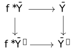
Let \mathcal {D} \to \mathcal {C} be a Grothendieck fibration. For every f: X \to Y, \bar {Y} \in \mathcal {D}_Y, select a Cartesian lift f^*\bar {Y} \to \bar {Y} of f.
Then there is a unique extension of f^* to a functor \mathcal {D}_Y \to \mathcal {D}_X so that the squares
commute. With this, the assignment X \mapsto \mathcal {D}_X, f \mapsto f^* assembles into a pseudofunctor \mathcal {C}^\mathrm {op} \to \mathsf {Cat}.
If \mathcal {D} \to \mathcal {C} is such that each morphism admits merely a locally Cartesian lift (but these do not compose,) it is called a prefibration. Note that this is unrelated to our notion of Markov prefibration (reading ahead a bit, the "Cartesian" maps in a Markov prefibration do compose, but they enjoy the unique lifting property only for a subset of morphisms). This clash of terminology is perhaps unfortunate, but other potential prefixes seemed inferior (quasi-, pseudo-, semi-).
Let \mathcal {C} be any category, and let \mathcal {C}^\to denote the arrow category. Then the codomain functor \mathcal {C}^\to \to \mathcal {C} is a fibration if and only if \mathcal {C} admits all pullbacks, and in this case the functors f^*: \mathcal {C}_Y \to \mathcal {C}_X, given f: X \to Y, are given by pullback along f.
The functors f^* are sometimes referred to as pullback, a convention we generally adopt. They are also sometimes called base-change functors.
When f: X \to Y and A \in \mathcal {D}_Y, we may write A_X for the object f^*A if there is no chance of confusion. (Compare that the choice of f is also suppressed in the notation A \times _Y X for a pullback)
We will not go into a comprehensive description of the theory of fibrations, but simply give a few basic results. We will give some examples in the next section. For a textbook treatment, see eg. Reference [jacobs-categorical-logic] (chapters 1, 9), or Reference [borceux-handbook] (chapter 8). Note that we will not give a formal definition of the term "pseudofunctor" here. See eg Reference [jacobs-categorical-logic], def. 1.4.4.
Let \mathcal {A}: \mathcal {C}^\mathrm {op} \to \mathsf {Cat} be a pseudofunctor. Then there is a category \int _{X \in \mathcal {C}}\mathcal {A}(X) defined as follows:
The objects are pairs {\bar {X}\in \mathcal {A}(X) \choose X \in \mathcal {C}}
The morphisms {\bar {X} \choose X} \to {\bar {Y} \choose Y} are pairs f: X \to Y, f^\#: \bar {X} \to \mathcal {A}(f)(\bar {Y}) \in \mathcal {A}(X)
Composition is given by the "chain rule" (f,f^\#) \circ (g,g^\#) = (fg, \mathcal {A}(g)(f^\#)g^\#)
There is an obvious forgetful functor \int _X \mathcal {A}(X) \to \mathcal {C}.
The category \int _X \mathcal {A}(X) is known as the Grothendieck construction of \mathcal {A}
Given f: X \to Y and \bar {Y} \in \mathcal {A}(Y), it is clear that the map {\mathcal {A}(f)(\bar {Y}) \choose X} \to {\bar {Y} \choose Y} given by f, 1_{\mathcal {A}(f)(\bar {Y})} is locally Cartesian---the required bijection is the definition of maps in the Grothendieck construction. But it's straightforward to see that these compose.
Given a pseudofunctor \mathcal {A}: \mathcal {C}^\mathrm {op} \to \mathsf {Cat}, it is obvious that the assignment \mathcal {A}(-)^\mathrm {op} is pseudofunctorial as well (the required natural isomorphisms are just the formal opposites of the ones for \mathcal {A}). Applying this through the equivalence of fibrations and pseudofunctors leads to the fiberwise opposite of a fibration. Explicitly:
Let p: \mathcal {D} \to \mathcal {C} be a fibration.
Then there exists a category \mathcal {D}^\mathrm {fop}, called the fiberwise opposite of \mathcal {D}, whose objects are the same as \mathcal {D}, and where a morphism X \to Y is a tuple (f: p(X) \to p(Y), f^\#: f^*Y \to X \in \mathcal {D}_{p(X)}).
We have already given somewhat of an account of lenses, optics, and their applications in the introduction. We briefly review the theory here, especially to normalize the notation and definitions. The best general source for this material is still Reference [riley-optics].
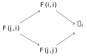
The definition of optic relies on the notion of coend, which we briefly recall, see Reference [fosco-coend-calculus] for a textbook account. If F: \mathcal {I}^\mathrm {op} \times \mathcal {I} \to \mathcal {C} is a functor, the coend\int ^{i \in I} F(i,i) is defined as the initial object receiving a map f_i : F(i,i) \to \int ^{i \in I} F(i,i) for each i \in I, so that for each \phi : i \to j, the square
commutes.
If \mathcal {C} has enough colimits, we may express the coend as the coequalizer of the diagram
\coprod _{f : i \to j \in \mathcal {I}} F(i,j) \rightrightarrows \coprod _{i} F(i,i),
where the two maps are given on each component by F(i,f): F(i,j) \to F(i,i) and F(f,j) : F(i,j) \to F(j,j), respectively. (This is Remark 1.2.4 in Reference [fosco-coend-calculus]). Note that in particular this implies that if \mathcal {C} has all colimits, then it also has all coends.
Let \mathcal {M} be a monoidal category which acts on two categories \mathcal {C}, \mathcal {D}. Then the category of optics\mathsf {Optic}_\mathcal {M}(\mathcal {C},\mathcal {D}) has
The set of morphisms {A \choose X} \to {B \choose Y} given by the coend
\int ^{M \in \mathcal {M}} \mathcal {C}(X, M \cdot Y) \times \mathcal {D}(M \cdot B,A)
Given two optics with representatives (M,f: X \to M \cdot Y,g : M \cdot B \to A), (N, f': Y \to N \cdot Z, g': N \cdot C \to B), their composite is given
by (M \otimes N, (1_M \cdot f')f, g (1_M \cdot g')), where we omit coherence morphisms.
When \mathcal {C} is a monoidal category acting on itself by tensor, we write \mathsf {Optic}_\mathcal {C}(\mathcal {C},\mathcal {C}) =: \mathsf {Optic}(\mathcal {C})
Note that if \mathcal {M},\mathcal {C},\mathcal {D} are symmetric monoidal and these actions are symmetric, \mathsf {Optic}_\mathcal {M}(\mathcal {C},\mathcal {D}) inherits a symmetric monoidal structure given by {A \choose X} \otimes {B \choose Y} = {A \otimes B \choose X \otimes Y}. (Also given a braiding one can induce a non-symmetric monoidal structure, but this almost never comes up).
Objects and morphisms in the category of optics have two parts---one going "forwards", in the same direction as the optic, and one going "backwards". In Reference [riley-optics] the objects are written (X,A), where X is the forwards part. Hedges' work on open games used the binomial notation \binom {X}{A}, but wrote the forwards part on top.
To make the connection to fibrations more natural, we instead write the forwards part on the bottom, {A \choose X}. It is the backwards part which depends on the forwards part, hence the forwards part is the base of the fibration (when one exists)---and every part of the language of fibrations is built around a mental model where the base is at the bottom and the fibers are over it (including the word "base"). When reading the references, this may cause some confusion, but hopefully this can be overcome.
While we're at it, let us note that when talking about optics we will freely use terms like "the forwards part" "the backwards object" and so on---the meaning of this should now be clear. Of course, once we get to cooptics/charts, this would be more than a little confusing, since in that case both components are in the same direction. In those cases we will speak of either the primary (forwards) part or the secondary (backwards) part, or use the language of fibrations and speak of the map or object "in the base" and "in the fiber".
As noted above, the coend \int ^M \mathcal {C}(X, M \cdot Y) \times \mathcal {D}(M \cdot B, A) consists of triples (M, f: X \to M \cdot Y, g: M \cdot B \to A) up to the equivalence relation which, for every \phi : M \to M', f: X \to M \cdot Y, g: M' \cdot B \to A, identifies the two tuples (M', (\phi \cdot 1_Y) f, g) and (M, f, g (\phi \cdot 1_B)). Note that this relation is not assumed to be inherently an equivalence relation---one takes the transitive-symmetric closure as usual.
We call this relation the sliding relation (because we slide the map \phi from the backwards part to the forwards part).
Suppose \mathcal {M}, \mathcal {C}, \mathcal {D} are small categories. Then the coend defining \mathsf {Optic}_\mathcal {M}(\mathcal {C},\mathcal {D})\left ( {A \choose X}, {B \choose Y} \right ) is a small colimit of small sets, hence again small. Since clearly the set of objects \operatorname {\mathbf {ob}} \mathcal {C} \times \operatorname {\mathbf {ob}} \mathcal {D} is small, \mathsf {Optic}_\mathcal {M}(\mathcal {C},\mathcal {D}) is again a small category.
However, if \mathcal {M},\mathcal {D},\mathcal {C} are merely assumed to be locally small, we can not guarantee the same is true of \mathsf {Optic}_\mathcal {M}(\mathcal {C},\mathcal {D}), since the hom-sets are now defined by a coend/colimit with large indexing category. However, in many special cases, it can still be seen to be locally small, such as in the Cartesian case (where \mathsf {Lens}(\mathcal {C}) is clearly locally small).
In this thesis, we will not delve further into this subtlety, simply working inside some universe where all our categories are small.
Of course, we can also let the arrows in \mathcal {D} go in the same direction as \mathcal {C}. This does not seem to have played any role in the literature, but we will give this a name, as it is a useful example to have in mind for Markov fibrations (where we will construct our dependent optics, conceptually, as a fiberwise opposite)
Given \mathcal {M} acting on \mathcal {C}, \mathcal {D}, the category of co-optics, \mathsf {coOptic}_\mathcal {M}(\mathcal {C},\mathcal {D}) has objects pair {A \in \mathcal {D} \choose X \in \mathcal {C}}, and morphisms given by the coend \int ^M \mathcal {C}(X, M \cdot Y) \times \mathcal {D}(M \cdot A, B)
For any monoidal category \mathcal {C}, \mathsf {Optic}_\mathcal {C}\left ({A \choose X}, {I \choose I}\right ) = \mathcal {C}(X,A). One way to think of an optic {A \choose X} \leftrightarrows {B \choose Y} is as a string diagram X \to A, but which has a hole with space for a morphism B \to Y. One inserts such a morphism by composing the optic with the optic {B \choose Y} \leftrightarrows {I \choose I} representing it. This idea of "open diagrams" has been developed in much more detail by Román, Reference [roman-optics-coend].
Suppose \mathcal {M} is semicartesian---in other words, that I \in \mathcal {M} is terminal. Then there is a functor \mathsf {Optic}_\mathcal {M}(\mathcal {C},\mathcal {D}) \to \mathcal {C}, which takes a {A \choose X} to X, and pair \langle f: X \to M \cdot Y, g \rangle to the composite X \to M \cdot Y \to I \cdot Y \cong Y.
In the case of \mathsf {Optic}(\mathcal {M}), the map \mathsf {Optic}(\mathcal {M})({I \choose I}, {A \choose X}) \to \mathcal {M}(I,X) is a bijection.
The fact that in \mathsf {Optic}(\mathcal {M}), states (maps from the monoidal unit) on {A \choose X} are given by states on X, while costates are given by maps X \to A plays an important role in the use of optics to describe open games. See § [efr-GFG0] for more on this.
Here we use a general fact about coends, that \int ^M \mathcal {C}(X,M) \times F(M) \cong F(X)---this has been called the ninja Yoneda lemma, see Reference [fosco-coend-calculus].
In this case we sometimes write \mathsf {Lens}(\mathcal {C}) for the category \mathsf {Optic}(\mathcal {C}). We have the following fact:
The functor {A \choose X} \mapsto X, \mathsf {Lens}(\mathcal {C}) \to \mathcal {C}, is a fibration. The fiber \mathsf {Lens}(\mathcal {C})_X has the following description:
Its objects are the objects of \mathcal {C}.
A map A \to B \in \mathsf {Lens}(\mathcal {C})_X is a map X \times B \to A \in \mathcal {C}.
The composite of X \times B \to A,X \times C \to B is given by composing the two into X \times X \times C \to A, then using the diagonal.
Given f: X \to Y, the pullback functor \mathsf {Lens}(\mathcal {C})_Y \to \mathsf {Lens}(\mathcal {C})_X is given by precomposing by f.
If \mathcal {C} moreover admits pullbacks, there is a fibred functor \mathsf {Lens}(\mathcal {C})^\mathrm {fop} \to \mathcal {C}^\to \to \mathcal {C}, which carries an object {A \choose X} to X \times A\xrightarrow {\pi _X} X, and a morphism f:X \times A \to B to the map X \times A \xrightarrow {\langle \pi _X,F \rangle } X \times B over X. This is fully faithful.
This is the first way to see the maps of (\mathcal {C}^\to )^\mathrm {fop} as dependent lenses---they receive the category of lenses as a full subcategory.
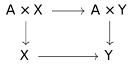
The squares
are pullbacks in any category with products, even if it does not admit pullbacks in general.
It follows that the full subcategory of \mathcal {C}^\to spanned by objects of this form is always a fibration over \mathcal {C}, which is isomorphic to \mathsf {coOptic}(\mathcal {C})---the fiberwise dual is isomorphic to \mathsf {Lens}(\mathcal {C}).
The basic idea of a Markov category is to interpret morphisms X \to Y as "stochastic processes" or kernels---that is, functions valued in probability measures. A morphism P \to X \otimes Y is a parametrized joint probability measure---the comonoid structure allows us to build a canonical such given parametrized measures P \to X, P \to Y (by precomposing their tensor with the \mathrm {copy}_P map). This is the product measure of the two---the fact that in general not every map has this form (because \mathcal {C} is not necessarily Cartesian) allows us to express the probabilistic dependence---as in, non-independence---of one variable on another.
A morphism is called deterministic if it is a comonoid (co)homomorphism, which amounts to the claim that \mathrm {copy}_Y f = (f \otimes f) \mathrm {copy}_X---in other words, that running two independent copies of the kernel (with the same input) is equivalent to running one and copying the output. The deterministic morphisms form a Cartesian monoidal subcategory which is denoted \mathcal {C}_\mathrm {det} \subseteq \mathcal {C}.
We first note the following alternative characterization of Markov categories in terms of their deterministic morphisms.
Let \mathcal {C} be a symmetric monoidal category. A premarkov structure on \mathcal {C} is a wide symmetric monoidal subcategory \mathcal {C}' \subseteq \mathcal {C}---that is, a class of morphisms which contains all identities and structural isomorphisms, and is stable under composition and monoidal products---so that the monoidal category \mathcal {C}' is Cartesian.
Given a premarkov structure\mathcal {C}' \subseteq \mathcal {C}, there is a unique Markov structure on \mathcal {C} so that each morphism in \mathcal {C}' is deterministic.
Given a Markov structure, \mathcal {C}_\mathrm {det} \subseteq \mathcal {C} is a premarkov structure.
A premarkov structure has the form \mathcal {C}_\mathrm {det} for some Markov structure if and only if it is maximal.
The existence part first claim is clear: \mathcal {C}' acquires a unique Markov structure since it is Cartesian, and the inclusion of that Markov structure into \mathcal {C} gives a Markov structure on \mathcal {C}. Conversely, suppose \mathcal {C} is a Markov category and \mathcal {C}' \subseteq \mathcal {C}_\mathrm {det} is a class of deterministic morphisms which is still Cartesian. This means the projections X \otimes Y \to X,Y still exhibit X \otimes Y as a product in \mathcal {C}'. But since the pairing are the unique map lifting two given maps A \to X,Y, the pairing must be preserved by the inclusion \mathcal {C}' \to \mathcal {C}_\mathrm {det}. Since the canonical Markov structure is given as a pairing, this means the markov structure induced by \mathcal {C}' \to \mathcal {C} must agree with the one given by \mathcal {C}_\mathrm {det}, which is just the original one.
Now suppose \mathcal {C}_\mathrm {det} \subseteq \mathcal {C}' \subseteq \mathcal {C}, where \mathcal {C}' is some larger premarkov structure. By the argument above, they must generate the same Markov structure on \mathcal {C}. But again, this implies that every map in \mathcal {C}' is deterministic for this Markov structure, so we have \mathcal {C}_\mathrm {det} = \mathcal {C}'. This finishes the proof.
Note that given a merely monoidal category, we can ask whether it is Cartesian, and if it is, it admits a unique symmetry induced by the universal property of the product. Hence if \mathcal {C}' \subseteq \mathcal {C} is a Cartesian wide monoidal subcategory, we may attempt to define a symmetry on \mathcal {C} simply using the one from \mathcal {C}'. However, it is not automatic that this symmetry is natural for all the morphisms in \mathcal {C}.
This basic idea was already noted by Fritz (and goes back to Golubtsov's work in Reference [golubtsov-kleisli], an important part of the prehistory of Markov categories), although the precise statement above appears to be novel. Since the coherence conditions required of the comonoids in a Markov structure can be somewhat hard to remember, this characterization may be easier to understand.
A Markov category is representable if the inclusion \mathcal {C}_\mathrm {det} \hookrightarrow \mathcal {C} admits a right adjoint. In this case we denote the right adjoint P and call the object PX for X \in \mathcal {C} a distribution object for X. Observe that \mathcal {C}(X,Y) = \mathcal {C}_\mathrm {det}(X,PY) (by definition,) and hence \mathcal {C} = Kl(P) where we denote the induced monad on \mathcal {C}_\mathrm {det}P by an abuse of notation.
\mathsf {Stoch} (Reference [fritz-synthetic-markov-cats], section 4) is the category whose objects are measurable spaces, whose morphisms are Markov kernels, with composition given by the Chapman-Kolmogorov equation and monoidal structure given by product measures.
\mathsf {BorelStoch} \subseteq \mathsf {Stoch} (Reference [fritz-synthetic-markov-cats], section 4) is the full subcategory of \mathsf {Stoch} spanned by the standard Borel spaces, that is by those measurable spaces arising as the Borel \sigma -algebra on separable, complete metric space.
\mathsf {FinStoch} is the subcategory of \mathsf {Stoch} spanned by finite sets in the powerset \sigma -algebra. A morphism X \to Y in \mathsf {FinStoch} is equivalently a matrix f_{xy} : x \in X, y \in Y with entries in \mathbb {R}_{\geq 0} and with \sum _y f_{xy} = 1 for each x (this is what is called a stochastic matrix).
Let \Delta : \mathsf {Set} \to \mathsf {Set} be the monad which assigns to X \in \mathsf {Set} the set \Delta (X) of countably-supported probability measures. Then the Kleisli category Kl(\Delta ) is a Markov category, sometimes called the category of discrete probability.
\mathsf {TychStoch} (Reference [markov-supports], example A.1.4) is the category of Tychonoff topological spaces and kernels which are valued in Radon probability measures, and where the measure f(- \mid x) varies continuous in x \in X with respect to the weak topology---in other words, given any continuous function u \in C(Y), the resulting function on X given by E_{y \sim f(- \mid x)}u(y) is continuous. (A space X is Tychonoff if it is Hausdorff and, given K \subset X closed and x_0 not in K, there exists continuous f: X \to [0,1] with f(x_0)=0, f(k) =1 for k \in K. Every locally compact Hausdorff space is Tychonoff).
If \mathcal {C} is a Markov category and I is any ordinary category, there is a Markov category \mathsf {Fun}(I,\mathcal {C}) whose objects are functors I \to \mathcal {C}_\mathrm {det}, and whose morphisms are natural transformations between these considered as functors into \mathcal {C} (i.e natural transformations with stochastic components). The monoidal and Markov structure is defined simply component-wise.
In particular, taking I = \to = \{0 \to 1\} the walking arrow, we obtain a Markov category of deterministic arrows \mathsf {Fun}(\to , \mathcal {C}). We will denote this category simply \mathcal {C}^\to . Again, the objects of this category are the deterministic morphisms of \mathcal {C}, while the morphisms are the commutative squares with not-necessarily-deterministic sides
When we speak of a stochastic map in a Markov category, we always mean a map which is not necessarily deterministic---that is, a general map of \mathcal {C}.
Given a map p: P \to X \otimes Y into a tensor product, the composites with the projections P \to X, P \to Y are called the marginals. Given two maps f: P \to X, g: P \to Y, we refer to any map P \to X \otimes Y with those marginals as a pairing of the two. Note that there is always a canonical pairing given by (f \otimes g) \mathrm {copy}_P. We write \langle f,g \rangle : P \to X \otimes Y for this canonical pairing. For deterministic maps this is just the usual pairing using the universal property of the product. (We mostly use this in cases where one map is deterministic, so that the pairing is unique assuming positivity). When p = \langle \pi _Xp, \pi _Yp \rangle , we say X \bot Y \mid P, and say the two coordinates are independent given P (or just independent).
Recall that the codomain functor \mathcal {C}^\to \to \mathcal {C} is a fibration if and only if \mathcal {C} admits pullbacks. Since Markov categories have terminal objects but not, in general, products, they clearly cannot be expected to have pullbacks.
However, if \mathcal {C} is positive (Reference [fritz-synthetic-markov-cats], def. 11.22---but see Proposition [efr-OYB6] below), given f: P \to Xdeterministic, every g: P \to Y has a unique pairing P \to X \otimes Y with f.
Computing pullbacks X \otimes _Z Y in the subcategory \mathcal {C}_\mathrm {det}, we usually have a similar property. This will be the basic idea behind Markov prefibrations.
By the following straightforward proposition, this property of having unique deterministic pairings is in fact equivalent to positivity:
PropositionCharacterization of positivity[efr-OYB6]
Let \mathcal {C} be a Markov category. The following are equivalent:
In \mathcal {C}, if f: P \to X \otimes Y has deterministic marginal P \to X, then X \bot Y \mid P. In other words, anything is independent of a deterministic variable.
Given a deterministic morphism P \to X and any morphism P \to Y, there is a unique P \to X \otimes Y with those marginals.
Clearly 1 and 2 are equivalent, since independence just means f is the independent pairing of the marginals---if it is uniquely determined by its marginals, it must be equal to the independent pairing, and conversely if it is necessarily independent, it is determined by its marginals. Now let us show this is equivalent to positivity.
First suppose \mathcal {C} has unique pairings in this sense. Let f,g be as in the definition of positivity. Then the two maps X \to Y \otimes Z indicated are pairings of gf and f, and since gf is deterministic, they are identical by hypothesis.
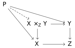
Let \mathcal {C} be a Markov category. We say \mathcal {C} is pullback-positive if \mathcal {C}_\mathrm {det} admits pullbacks and, given a diagram of this form where P \to X is deterministic, there is a unique map P \to X \times _Z Y making the squares commute.
Note that a pullback-positive category is in particular positive by taking Z = I.
The pullbacks appearing in Definition [efr-T3HM] are of course pullbacks in \mathcal {C}_\mathrm {det}, not \mathcal {C}, analogously to how X \otimes Y is a product in \mathcal {C}_\mathrm {det}, not \mathcal {C}. We will still use the notation X \times _Z Y for these pullbacks, which should not lead to any confusion. We may occasionally write X \times Y instead of X \otimes Y, if we are carrying out a construction which primarily involves \mathcal {C}_\mathrm {det}. Since essentially no Markov categories have Cartesian products (except when the tensor product is Cartesian), this should also not lead to any ambiguity.
Suppose any category \mathcal {C}' admits products and intersections---that is, pullbacks U \times _X V whenever U,V are subobjects of X. Then it admits all finite limits.
Suppose \mathcal {C}_\mathrm {det} admits and \mathcal {C}_\mathrm {det} \to \mathcal {C} preserves pullbacks along monomorphisms. Suppose further \mathcal {C} is positive. Then it is pullback-positive.
To see the first point, let f: X \to Z, g: Y \to Z be arbitrary maps. Note that X \times _Z Y = (X \times Y) \times _{X \times Y \times Z \times Z} X \times Y \times Z, where the horizontal map is given by (x,y) \mapsto (x,y,f(x),g(y)), and the top by (x,y,z) \mapsto (x,y,z,z)---in the sense that the universal property of this intersection is exactly the universal property of the given pullback.
Now suppose \mathcal {C}_\mathrm {det} \to \mathcal {C} preserves this intersection, and \mathcal {C} is positive. (Note that it doesn't follow that the inclusion preserves the pullback X \times _Z Y, because it doesn't preserve the products). This amounts to the claim that a map P \to X \otimes Y lifts to the pullback if and only if the composite P \to X \otimes Y \otimes Z \otimes Z lifts over the map 1_X \otimes 1_Y \otimes \mathrm {copy}_Z (note that the pullback of a monomorphism is a monomorphism).
This implies in particular such a lift is always unique. Since if \mathcal {C} is positive, given P \to X, P \to Y, if the latter is deterministic there is a unique pairing P \to X \otimes Y, this implies there is at most one map P \to X \times _Z Y pairing the two. On the other hand, since the composite P \to Y \to Z is deterministic and equal to the composite P \to X \to Z, they are both deterministic, and hence the pairing P \to Z \otimes Z factors over the diagonal. Applying positivity again, to the tensor product (X \otimes Y) \otimes (Z \otimes Z), since the latter component is deterministic, this pairing is independent, and hence the map P \to X \otimes Y \to X \otimes Y \otimes Z \otimes Z does indeed lift, finishing the proof.
The idea here is that a distribution on a subobject X' \subseteq X defined by some condition f(x \in X) \in U \subseteq Y is simply a distribution so that the condition is satisfied with probability 1. This is a natural condition which holds in many Markov categories.
The assumption that \mathcal {C} is pullback-positive will play a key role in the development of the theory of Markov fibrations. Although the theory could possibly be developed without assuming the base category has deterministic pullbacks, positivity seems to be an essential part.
If \mathcal {C} is representable and positive, \mathcal {C}_\mathrm {det} has limits, and the monad P preserves intersections, then \mathcal {C} is pullback-positive.
This is clear, since if the monad P preserves a given limit, so does the inclusion into the Kleisli category (for completely abstract reasons), hence by Lemma [efr-0YP1] we are done.
We will need the notion of support in a Markov category, introduced in Reference [markov-supports], for certain examples, so we briefly record the definition and a few of its properties here.
Let p: X \to Y, q: A \to Y be two morphisms in a Markov category. We say q is absolutely continuous with respect to p and write q << p if, whenever two maps Y \to Z are p-almost surely equal, they are also q-almost surely equal.
Let p: X \to Y be a morphism in a Markov category. The support of p, if it exists, is an object which represents the functor \mathcal {C}(-,Y)_{<<p} of morphisms into Y which are absolutely continuous with respect to p.
The support of p: X \to A is equipped with a canonical deterministic monomorphism S_p \hookrightarrow A, so that a map into A is absolutely continuous with respect to p if and only if it factors over the support.
Two maps A \otimes W \to B are p-almost surely equal if and only if they are strictly equal on the support.
A (strict) double category is a category internal to the category \mathsf {Cat} of categories.
Concretely, it consists of:
A set of objects \operatorname {\mathbf {ob}} \mathbb {C}
A collection of vertical morphisms forming a category \mathbb {C}_v with \operatorname {\mathbf {ob}} \mathbb {C}_v = \operatorname {\mathbf {ob}} \mathbb {C}
A collection of horizontal morphisms forming a category \mathbb {C}_h with \operatorname {\mathbf {ob}} \mathbb {C}_h = \operatorname {\mathbf {ob}} \mathbb {C}
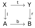
An a collection of squares. Each square has a left and right boundary given by vertical morphisms l,r, and top and bottom boundary given by horizontal morphisms t,b so that \operatorname {\mathrm {dom}} t = \operatorname {\mathrm {dom}} l, \operatorname {\mathrm {cod}} t = \operatorname {\mathrm {dom}} r and so on:
The squares compose horizontally and vertically in the obvious way, each of which form a category (in particular, there are identity squares for each vertical and horizontal map).
A double functor is a mapping on objects, vertical and horizontal morphisms, and squares, which preserves all the identities and composition.
There is also a notion of pseudo double category, which weakens the horizontal composition to only be associative and unital up to a coherent system of squares. We will not go into the details here, see § [efr-000D] for more on this.
There is a pseudo double category \mathsf {\mathbb Cat} where the objects are categories, the vertical maps are functors, the horizontal maps are profunctors (functors \mathcal {C} \times \mathcal {D}^\mathrm {op} \to \mathsf {Set}, sometimes called bimodules), and the squares are natural transformations.
For any category with pullbacks \mathcal {C}, there is a pseudo double category \mathsf {\mathbb Span}(\mathcal {C}) with \mathcal {C} as the vertical category, spans as the horizontal morphisms, and commutative diagrams as the squares.
There is a double category \mathsf {\mathbb Rel} of sets, functions, and relations.
For any Markov category \mathcal {C}, there is a double category with \mathbb {C}_v = \mathcal {C}_\mathrm {det} and \mathbb {C}_h = \mathcal {C}.
For any category at all, there is a double category \operatorname {Sq}(\mathcal {C}) with \operatorname {Sq}(\mathcal {C})_v = \operatorname {Sq}(\mathcal {C})_h = \mathcal {C} and commutative squares as the pullback squares.
A double category is thin if, for each compatible square of vertical and horizontal morphisms, there is at most one square filling it. In other words, such a square either commutes or doesn't.
Sometimes the two classes of morphism are instead called loose and tight, especially in cases where the composition of the loose class is not associative, or if the loose class is a superset of the tight class.
Although the explicit description above is probably the best way to think about the data of a double category, on a technical level it is often useful to think in terms of internal categories. An internal category in a category \mathcal {C} is a pair of objects C_0, C_1, maps d,c: C_1 \to C_0, i: C_0 \to C_1 (the domain, codomain and identity), and a map m: C_1 \times _{C_0} C_1 \to C_1 (the multiplication), satisfying the usual laws of a category. A double category in the above sense is then an internal category in the category of categories.
In the terms of Definition [efr-RXP4], C_0 is \mathbb {C}_v, and C_1 is the category whose objects are horizontal arrows, and whose morphisms are squares (composed vertically). Obviously, we could just as easily have oriented things horizontally, but this is the convention usually adopted.
Given a double category \mathbb {C}, there is another double category \mathbb {C}^T called the transpose of \mathbb {C}, which has the same objects but exchanges the horizontal and vertical morphisms. In many cases it is not clear which of \mathbb {C} and \mathbb {C}^T is the "correct" one to work with, and we may have to pass back and forth between them. We try to stick to the convention that the horizontal morphisms are the "loose" ones. To avoid confusion, we will also simply specify the classes of morphisms directly, speaking for example of "the lenses" or "the charts" when working with the double category \mathsf {\mathbb Arena}(\mathcal {A}) (Definition [efr-0025]).
The concept of double category goes back to Reference [ehresmann-dblcats]. See Reference [johnson-yau-2dim-categories], section 12.3 for a textbook treatment. They have been widely used in applied category theory. An early application is in Reference [baez-courser-structured-cospans], which constructed a "structured" version of the double category of cospans. Here the philosophy is that the horizontal morphisms are the "systems" (in a general sense) which are being wired together by horizontal composition, while the vertical morphisms (and squares) are "structure-preserving maps between systems". This is similar to the our double category of "bisystems" (§ [efr-MWCE]). Recent work by Lambert and Patterson Reference [patterson-lambert-dbltheory] applies double categories to categorical algebra, with many applications to systems modeling, see Reference [catcolab-introducing] (as well as to classical category theory). In the next section we'll see their application to categorical systems theory, and later see them applied to parametrized morphisms.
A theory of dynamical systems is an indexed category \mathcal {A}: \mathcal {C}^\mathrm {op} \to \mathsf {Cat} equipped with a section of its Grothendieck construction T: \mathcal {C} \to \int \mathcal {A}.
It is called monoidal if \mathcal {C} is a monoidal category, and \mathcal {A} is a lax monoidal functor. It is further called symmetric monoidal if \mathcal {C} is a symmetric monoidal category and \mathcal {A} is a symmetric lax monoidal functor. Note that this is equivalent to requiring \int \mathcal {A} \to \mathcal {C} to be a (symmetric) monoidal fibration in the sense of Reference [shulman-monfibs] (see also Reference [moeller-vasilakopoulou]).
Let \mathcal {A}: \mathcal {C}^\mathrm {op} \to \mathsf {Cat} be an indexed category. A chart is simply a morphism in the Grothendieck construction \int \mathcal {A}. A lens is a morphism in the fiberwise opposite \int \mathcal {A}(-)^\mathrm {op}.
Given an indexed category \mathcal {A}: \mathcal {C}^\mathrm {op} \to \mathsf {Cat}, the double category \mathsf {\mathbb Arena} of arenas has
Objects the objects of \int \mathcal {A}---note that these are the same as the objects of \int \mathcal {A}(-)^\mathrm {op}
Vertical morphisms the lenses
Horizontal morphisms the charts
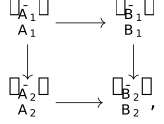
The double category is thin. Given a square of this form
we can first project it to a square in \mathcal {C}. If this commutes, we can pull the lenses and charts back to a square in \mathcal {A}(A_1). The above square of lenses and charts will be said to commute if both of these squares commute.
We will write arenas either as {\bar {A} \in \mathcal {A}(A) \choose A \in \mathcal {C}}, or, for brevity when there is no need to discuss the two levels separately, simply with a symbol A. We will also write both {\bar {TS} \choose S} and TS as the situation calls for---there should be no confusion resulting from this.
DefinitionDynamical system with interface A[efr-0028]
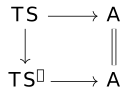
Let A be an arena. A dynamical system with interface A is an object S \in \mathcal {C} and a lens TS \leftrightarrows A. A morphism of systems is a map S \to S' so that this square commutes in \mathsf {\mathbb Arena}:
The category of systems with interface A is denoted \mathsf {Sys}(A)
Given a lens A \leftrightarrows A', postcomposition gives a functor \mathsf {Sys}(A) \to \mathsf {Sys}(A').
Given a chart A \rightrightarrows A', there is a profunctor\mathsf {Sys}(A) \nrightarrow \mathsf {Sys}(A'),
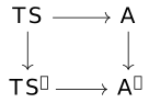
where the set over TS \leftrightarrows A and TS' \leftrightarrows A' is the set of maps S \to S' so that this square commutes:
This defines a double functor \mathsf {Sys}: \mathsf {\mathbb Arena} \to \mathsf {\mathbb Cat}.
The fibration \int \mathcal {A} \to \mathcal {C} encodes what sort of information can be "indexed over a space", while the section T: \mathcal {C} \to \int \mathcal {A} tells us what sort of information (such as a next step, or a gradient vector) must be produced to give a dynamical system. In this respect, the theory is very similar to the coalgebraic approach to dynamical systems, or systems that "do something", and indeed we have the following:
Let F: \mathsf {Set} \to \mathsf {Set} be a functor.
Then there is a dynamical systems theory where \mathcal {C} = \mathsf {Set}, \mathcal {A} is constant at \mathsf {Set},
and T(X) = (X,F(X)). It is easy to see that the category of closed dynamical systems in this theory is equivalently the category of F-coalgebras.
Of course, coalgebras can already encode systems with input and output---the point of the CST framework is to separate out the input and output of systems so that they can be acted on in a compositional manner.
ExampleThe theory of discrete dynamical systems[efr-002F]
There is a theory of dynamical systems with category of spaces \mathcal {C} = \mathsf {Set}, category of bundles \mathcal {A}(X) = \mathsf {Set}_{/X} (with pullbacks for reindexing), and tangent bundle TX = X \times X \xrightarrow {\pi _0} X.
We call this the theory of discrete dynamical systems. (In the sense that they are both discrete-time and discrete-space).
In another direction, we have the following comparison result:
The category of lenses \int \mathcal {A}(-)^\mathrm {op} is equivalently the category of polynomial functors and natural transformations between them.
Using this equivalence, the category of dynamical systems with interface p is exactly the category of p-coalgebras and homomorphisms
The first part here (which works, suitably formulated, for any locally Cartesian closed category), is a classical part of the theory of polynomial functors, see eg Reference [kock-poly-classical]. The second part is due to Spivak, see Reference [spivak-poly-abundant]. There is an extensive body of work on the description of interacting (discrete, deterministic) dynamical systems in terms of polynomial functors, see e.g. also Reference [shapiro-spivak-dynamic-operads].
ExampleThe theory of stochastic discrete dynamical systems[efr-GXJ0]
There is a systems theory where \mathcal {C} = \mathsf {Set}, \mathcal {A}(X) = Kl(\Delta )^X (with the evident reindexing maps) and T(X) = X \times X.
In this theory, a closed dynamical system is a set equipped with a map X \to \Delta (X). An open dynamical system has stochastic update function, but output which depends deterministically on the current system state.
In fact this example works for any monad on the category of sets.
ExampleThe theory of smooth dynamical systems[efr-KZEM]
There is a dynamical systems theory where \mathcal {C} = \mathsf {SmMfd} is the category of smooth manifolds, \mathcal {A}_X is the category of fiber bundles over X, with f^*: \mathcal {A}_Y \to \mathcal {A}_X given by pullback along f: X \to Y (note that pullbacks of bundles always exist), and with TX being the tangent bundle of X in the ordinary sense. In this case, closed dynamical systems are manifolds equipped with (smooth) vector fields, which is what is classically thought of as a smooth dynamical system.
Consider the theory of discrete-time, discrete dynamical systems from Example [efr-002F]. Let \xi : TS \leftrightarrows {I \choose O} be a system.
Consider the system c: T\mathbb {N} \leftrightarrows {* \choose \mathbb {N}} given by n \mapsto n in the forwards direction, and (n,*) \mapsto n+1 in the backwards direction. (To be clear, the object denoted {* \choose \mathbb {N}} is the map \mathbb {N} \to \mathbb {N}---it is a singleton in each fiber). Then a morphism of systems c \to \xi consists of the following data:
A function x: \mathbb {N} \to S.
Another function o: \mathbb {N} \to O.
A third function i: \mathbb {N} \to I so that i(n) \in I_{o(n)}.
So that o(n) = \xi (x(n)) and \xi ^\#(x(n),i(n)) = x(n+1)
That is, it is a choice of a sequence x_n of points in the state-space, and a sequence of inputs i_n compatible with the outputs, so that this sequence obeys the dynamics. In other words, it is a trajectory of the system.
Because of this, one views a generic chart map as a generalized trajectory, of a type given by the domain system. As another example, taking the state space to be \{1,2, \dots , n\} with an update map that carries n to 1, one finds a system which classifies n-periodic trajectories. Similarly, in the smooth case, the system (\mathbb {R}, d/dt: \mathbb {R} \to T\mathbb {R}) classifies solutions of a smooth differential equation (those which extend to infinity).
Recent work by Lynch, Myers, Staton, and the author (Reference [lynch-myers-rischel-staton-stoch-clocks]) constructs clock systems for theories of stochastic, discrete-time doctrines, although we will not delve into this here.
Because this thesis is about Markov fibrations, we have chosen to present these ideas in terms of fibrations equipped with sections. Myers' book Reference [myers-cst] actually prefers the presentation in terms of indexed categories. Similarly, we construct a double category of systems which is fibred (in a certain sense) over the double category of arenas. Myers instead displays this as a doubly indexed category\mathsf {\mathbb Arena} \to \mathsf {\mathbb Cat}, which carries lenses to functors and charts to profunctors.
In a recent paper Reference [double-operadic-systems], Myers and Libkind further develop the category theory of what they term double operadic categorical systems theory, which again concerns notions of "composable system" which are described in terms of such doubly indexed category (although for technical reasons, they use the language of right modules in that paper and a somewhat different presentation, the concept is the same.)