Free Markov Prefibrations [efr-GO6R]
Free Markov Prefibrations [efr-GO6R]
Because every map in Kl(\Delta )^\to factors into arrows which are "induced" from arrows in Kl(\Delta )^\to |_\mathrm {det} and the Markov prefibration property, it may initially be hoped that Kl(\Delta )^\to is in some sense "free" on the data of the fibration Kl(\Delta )^\to |_\mathrm {det} \to \mathsf {Set} and the inclusion \mathsf {Set} \to Kl(\Delta ). If that was true, we may further hope that taking the fiberwise opposite of the fibration and applying the same free generation principle would generate a good notion of stochastic lens.
Unfortunately, this is not the case. We will see that the free prefibration is given by gadgets which look a bit like an indexed version of optics, up to a sliding equivalence for deterministic maps on the residual. This prompts us to look for some extra structure on the fibration \mathcal {D}|_\mathrm {det} \to \mathcal {C}_\mathrm {det} which describes sliding equivalences for stochastic maps on the residual. In the next section, we will see that this is exactly the structure of an Eilenberg-Moore algebra for the free prefibration monad on \mathsf {Fib}(\mathcal {C}_\mathrm {det}).
In this section, we will give a description of the free Markov prefibration on a fibration \mathcal {D}_0 \to \mathcal {C}_{\mathrm {det}} (assuming \mathcal {C} is pullback positive). There is a fairly simple description of the hom-sets, but their composition is a bit tricky, and verifying associativity even more so. Hence we will employ a technical trick: by characterizing the hom-sets as "freely generated" in a certain sense from the hom-sets in \mathcal {D}_0, we can identify them with sets of natural transformations using a Yoneda-type argument, and infer composition and associativity from there.
Of course, there is a dual notion of indexed presheaf, but this will not interest us.
The idea of our construction of the free Markov prefibration is to give a certain monad on \mathsf {IcoPSh}(\mathcal {D}_0 / \mathcal {C}) and consider the Kleisli maps between the representable copresheaves.
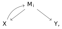
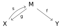
At this point, the notion of a deterministic map M \to X equipped with a stochastic (ie not necessarily deterministic) section begins playing a key role. The phrase "stochastic section" will always carry an implicit "of a deterministic map". In most cases the map that the section is a section of will be clear from the context.
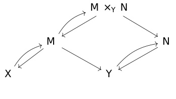
Note that, given a stochastic section Y \to M and a deterministic map X \to Y, if \mathcal {C} is pullback-positive, there is a unique lifting of this to a section of the projection Y \times _X M \to Y. We will use this fact several times.
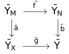
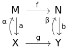
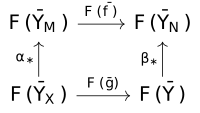
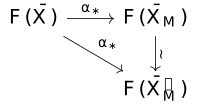
The term "stochastic module" is not very good, but this is mostly a nonce definition in any case, so we won't worry too much about it.
Stochastic modules over a given X \in \mathcal {C} can be seen to be monadic over the category of indexed copresheaves over that X. However, the compatibility of these local left adjoints with the structure of the rest of the category is somewhat subtle. However, we do have free stochastic modules on representable indexed copresheaves, as we will soon see.
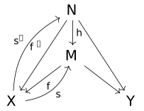
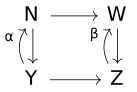
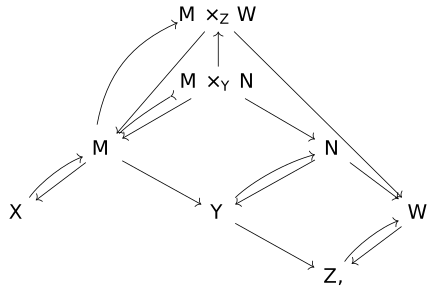
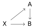
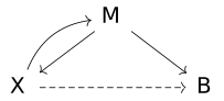
We are now ready to prove the main proposition of this section:
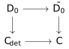
This characterization of the left adjoint makes it fairly easy to understand the induced monad on \mathsf {Fib}(\mathcal {C}_\mathrm {det}).
It is immediately obvious that we have:
Let us try to understand the structure of a stochastic module fibration. It is easiest to understand in the case of a projection map P \times X \to X. Suppose we have two objects A,B over X. Then we think of a map f: \pi _X^*A \to \pi _X^*B over P \times X as a map P \times A \to B, that is a map parameterized by P (this is literally the case for a codomain fibration). Given a stochastic section s of \pi _X, which amounts to a stochastic map X \to P, the stochastic module stucture picks out a new map s_*f, which is given over each point x \in X by choosing the parameter according to s, then applying f.
The definition of the composite in Proposition [efr-A08L], in these terms, tells us that given maps f: P \times A \to B, g: Q \times B \to C, and maps s: X \to P, t: X \to Q, the composite of s_*(f) and t_*(q) is equal to the map obtained by forming the parameterized composite Q \times P \times A \to C and applying the independent pairing \langle t,s \rangle : X \to Q \times P. This is of course how composition is supposed to work in a Markov category.
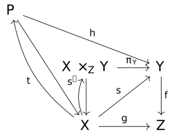
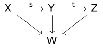
By construction, two morphisms in \overline {\mathcal {D}}_0 represented by spans with apex M,M', are identified if there exists a zig-zag M \to K_0 \leftarrow K_1 \to \cdots \leftarrow M' of spans (decorated with sections from the domain X and morphisms in the fiber, satisfying equations, etc). We will now prove a lemma that allows us to cut this down to a smaller set in many conditions. We will need the following hypothesis:
Observe that, if \mathcal {C} admits conditionals, it certainly admits weak conditionals: given a pullback X \times _Z Y, and maps P \to X,Y, form a Bayesian inverse of Y \to Z with respect to the given measure, and use that to build a lifting X \to Y, which gives X \to X \times _Z Y---then a diagram chase verifies that this map has the desired properties.