Let \mathsf {CartSp} denote the full subcategory of \mathsf {SmMfd} spanned by the objects \mathbb {R}^n for each n. Note that \mathsf {CartSp} has finite products, and is generated by the object \mathbb {R} under finite products.

A smooth space is a sheaf on \mathsf {SmMfd} in the standard topology of open covers. A smooth space X is a diffeological space if, for each M \in \mathsf {SmMfd}, the map X(M) \to \prod _{p \in M} X(\{p\}) is injective.

A diffeological space with underlying set X is called a diffeology on X, and consists of specifying which maps \mathbb {R}^n \to X are smooth. We call these maps smooth plots.

Given a subset X' \subset X, there is an obvious canonical diffeology on X' given by taking the plots to be those functions whose image in X is smooth. We call this the subspace diffeology.

A morphism of diffeological spaces is called a smooth map. It is equivalently a function X \to Y which carries smooth plots to smooth plots.

A diffeo-topological space is a diffeological space X equipped with a topology \tau so that all the smooth plots are continuous. A map of diffeo-topological spaces is a smooth map (for the diffeology) which is also continuous (for the topology).

Given a subset X' \subset X, there is an obvious canonical diffeo-topology on X' given by taking the plots to be those functions whose image in X is smooth, and equipping X' with the subspace topology.

The category of diffeo-topological spaces admits all limits, given by taking the limits in topological spaces and diffeological spaces (which have the same underlying set).

Let X be a diffeo-topological space whose underlying space is Tychonoff. Then the space of probability measures P(X) has a canonical diffeology given by those plots f: U \to P(X) so that for each continuous function g on X, the resulting map u \mapsto E_{f(u)g} is continuous, and if g is smooth, then this is smooth as well. With this diffeology, and the topology of weak convergence, P(X) is a diffeo-topological space. This defines a commutative affine monad on \mathsf {TychDiff}, the category of such diffeo-topological spaces.

Proof

• May 2, 2025
• Eigil Fjeldgren Rischel

The topology of weak convergence on P(X) is such that A \to P(X) is continuous if and only if the expectation map carries continuous functions to continuous functions. But this is part of the requirement to be a smooth plot, so certainly this is a diffeo-topological space.

Since the linear operator associated to x \in X under the unit X \to P(X) is merely evaluation at x, the unit is clearly smooth. Consider \mu : PPX \to PX. To test this is smooth, let f: U \to PP(X) be a plot. We must show \mu f is a plot. So let v: X \to \mathbb {R} be a continuous (resp. smooth) function. We must show its expectation a is continuous (resp. smooth) function of u \in U.

By construction E(v) : PX \to \mathbb {R} is continuous (resp. smooth), and so since f is a plot, the map u \mapsto E_{f(u)}E(v) is continuous (resp. smooth). But this is exactly what we wanted.

The monad laws follow from their holding in \mathsf {Tych}. Since a commutative monad is equivalently a strong monad satisfying a certain equation (which holds for this monad in \mathsf {Tych} and therefore also here), it suffices to show that the strength P(X) \times Y \to P(X \times Y) is smooth. This follows by a completely analogous argument.

The category \mathsf {TychDiffStoch} of Tychonoff diffeological spaces and Kleisli maps for the monad P described in Proposition [efr-7RS2] is a pullback-positive Markov category. Its deterministic category is \mathsf {TychDiff}. There is a fully faithful functor \mathsf {SmMfd} \to \mathsf {TychDiff} which preserves transverse pullbacks. The maps between smooth manifolds are given by weakly continuous families of Radon probability measures, so that the expectation operator carries smooth maps to smooth maps.

Since we describe properties of kernels in terms of their corresponding linear operator on function spaces, it would seem natural to take the function spaces as the basic object. Hence we might consider the category C^\infty -algebras with some relaxed notion of maps between them. The tricky part there is to find some reasonable class of maps so that the tensor product (coproduct) of C^\infty -algebras extends to these. (Since it is not the same as the tensor product of \mathbb {R}-algebras, linear maps do not automatically extend to the tensor product). In particular, when considering kernels *_1 \to X where *_1 is a "fat point of order 1"---that is, functions on 1_* have a value at the point and a derivative---it is not clear what sort of continuity condition the derivative operation on C^\infty (X) should satisfy, nor how to define this in a general way for all C^\infty -algebras. It would certainly be of interest to synthetic computational geometry to have such a Markov category, but we leave this for future work.

Consider the Markov prefibration \mathsf {TychDiffStoch}^\to \to \mathsf {TychDiffStoch}. Equip this with the section T(X) = X \otimes X \xrightarrow {\pi _0} X - this described discrete-time systems (whose update is required to be smooth in the input and present state). This is clearly a symmetric monoidal functor and thus defines a systems theory. Note that this is completely different from the ordinary tangent bundle, despite the coincidence of notation.

Let m_1: TS_2 \otimes X_1 \leftrightarrows Y_1 and m_2: TS_2 \otimes X_2 \leftrightarrows Y_2 be two bisystems in this theory. As in § [efr-SREZ], we may define a parameterized lens (TS_1 \& TS_2) \otimes (X_1 \oplus X_2) \leftrightarrows (Y_1 \oplus X_2), denoting by \oplus the coproduct in lenses, and by \& the Markov structure defined in Corollary [efr-FT8J]. Observe that TS_1 \& TS_2 is simply the indexed set (S_1 \coprod S_2) \otimes S_1 \otimes S_2 \to S_1\otimes S_2. There is an obvious indexed map from this to T(S_1 \otimes S_2) = S_1 \otimes S_2 \otimes S_1 \otimes S_2, given by (\operatorname {inl} s_1', s_1,s_2) \mapsto (s_1', s_2, s_1, s_2) and (\operatorname {inr} s_2', s_1, s_2) \mapsto (s_1,s_2',s_1,s_2). In words, we receive an update either to the S-state or to the S'-state. We apply this update to the relevant state and leave the other alone. This defines a lens T(S_1 \otimes S_2) \leftrightarrows T(S_1) \& T(S_2), which we may compose with the above to obtain a bisystem T(S_1 \otimes S_2) \otimes (X_1 \oplus X_2) \leftrightarrows Y_1 \oplus Y_2. Let us denote this by m_1 \oplus m_2.

This has very much the same flavor as the external choice for open games, although we will not develop the theory of this operation in detail here.

Now, given a smooth (deterministic) map F: P \times X \to Y, where P,X,Y are smooth manifolds (not merely diffeo-toplogical spaces), we obtain a lens T^*(F): {T^*P \choose P} \otimes {T^*X \choose X} \leftrightarrows {T^*Y \choose Y}, where T^*(-) denotes the cotangent bundle. (This does not, prima facie, make sense for a general diffeo-topological space).

Let us take as given some family of lenses T(S) = {S \otimes S \choose S} \leftrightarrows {T^*S \choose S} for various S. Such an operation amounts to choosing a way of updating s \in S given a cotangent vector---hence we can see it as an optimization algorithm. One example of such would be gradient descent, which given a choice of Riemann structure on S, takes a step of a given length in the direction which most quickly decreases the given covector.

(It should be noted that there are more complicated optimization strategies which don't fit this particular pattern - for example, momentum algorithms have to maintain some extra internal state other than s \in S. But let's stick with this pattern for this example). Note also that we're not assuming the optimizers are a natural transformation or anything like that.

Now we are ready to build the neural network architecture known as a generative adversarial network, or GAN (Reference [gan-paper]). Let us first describe the idea. Our goal is to generate additional samples from some distribution, given a set of existing samples---for example, our goal may be to generate more pictures in the same style as an existing corpus. Suppose our data is of type X, and let d: I \to X be the data distribution. We fix some latent distribution \lambda : I \to L, where L is any space of our choice---usually, L is \mathbb {R}^n and \lambda is a Gaussian. Finally we choose two neural networks, the generator G: P_G \otimes L \to X, and the discriminator D: P_D \otimes X \to \mathbb {R}. The goal of the discriminator is to discriminate real samples from the data from generated samples, by providing a low value on the generated samples and a high value on the true samples.

The training process now goes as follows: for each step of training, we either sample from the latent distribution, and have the generator use this to generate a sample, or draw a sample from the data distribution (choosing between these with some probability p). Then in either case, we have the discriminator score the generated sample. If the sample was generated by the generator, the discriminator's loss is equal to its output, otherwise it is equal to -1 times its output. We update the discriminator according to the gradient of this loss (minimizing it), and update the generator (if we are in the branch where it was run) according to the negative of the gradient of this loss with respect to the generator parameters---this amounts to doing a gradient descent update on the generator for the negative of the discriminator loss.

We can represent this schematically using the following tape diagram (see Reference [tape-diags-monoidal-monads]):

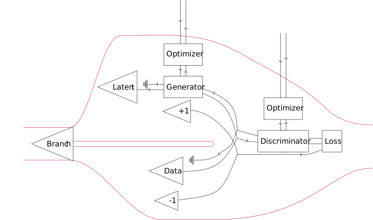
The two "tapes" branching off at the start represent two maps (bisystems) composed by \oplus , while the backwards wires indicate the flow of the gradients. The ground symbol indicates a value being discarded. Note that the theory of tape diagrams has only been developed formally for distributive categories, and for essentilly the same reason as in § [efr-SREZ], we do not have distributivity in this case. However, the interpretation of this diagram is still unambiguous---distributivity is required to make tape diagrams complete, not to make them sound. Concretely, if we tried to represent the tensoring of this system with another system, we would have no way of doing it, but if the category was distributive we could do so by adding this additional system to each of the branches. Still, the figure is best viewed as a visual aid rather than a formal representation.