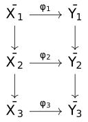
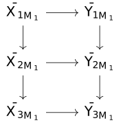
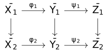
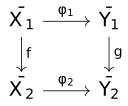
Given a set of inputs A and a set of outputs B, there are essentially two make sense of the informal description "finite-state automaton which reads inputs from A and produces outputs in B".
These are the notions of Mealy machine and Moore machine. Simply put, if the set of states is S, a mealy machine is a function A \times S \to B \times S, whereas a Moore machine is a pair A \times S \to S, S \to B. In other words, in a Moore machine the output does not depend on the current input, but only on previous inputs (through their effect on the state), but in a Mealy machine, the input can be passed through directly.
Using the language of categorical systems theory, we can make the following definitions:
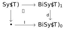
In a dynamical systems theory, a Moore machine with state space S and interface A is a lens TS \leftrightarrows A. The category of Moore machines with interface A is the slice category of the functor T over A---that is, a morphism of Moore machines is a morphism S \to S' so that the obvious triangle commutes.
In a dynamical systems theory, a Mealy machine with state space S and interface A consists of a costate lens TS \otimes A \leftrightarrows I. The category of Mealy machines with interface A is the comma category of the functor T(-) \otimes A over I---that is, a morphism of Mealy machines is S \to S' so that the obvious triangle commutes.
A Moore machine in the sense of Definition [efr-0006] is what Myers calls a (open) dynamical system, and they are the central object of study in Reference [myers-cst]. Arguably, both Moore machines and Mealy machines deserve the name of "open dynamical system"---the difference is how they interact with the external world.
Observe in particular that, if A=I, the categories of Mealy and Moore machines agree, both being equal to the slice of T over the unit I. In other words, the two notions of closed dynamical system coincide.
It is clear that both Mealy and Moore machines, in this sense, are special kinds of parametrized morphism in lenses, namely those parametrized by an object of the form TS. This leads naturally to the idea that there should be a triple category of morphisms of this type, charts, and lenses.
We call the parametrized lenses TS \otimes \bar {A} \leftrightarrows \bar {B}bisystems since they generalize the two types of machine, Moore and Mealy (but we choose to stick with "system" rather than "machine").
Wanting to learn a function X \to Y, we choose a parametrized function f: X \times P \to Y, where all these are, in the simplest case, Euclidean spaces \mathbb {R}^k
We take the backwards derivative of f, obtaining a lens:(f,Df): {TX \choose X} \otimes {TP \choose P} \leftrightarrows {TY \choose Y}
For each datum (x_n,y_n), we compute the loss gradient \nabla L(-,y_n) : Y \to TY, and combining this with x_n \in X and the current parameter p, we get a gradient on the parameter space which we can use to update
Thus a machine learning algorithm is a sort of bisystem. Indeed our bisystems are essentially an abstracted version of the learners of Fong--Spivak--Tuyeras. The functoriality of this assignment is the main point of the above-mentioned papers.
In this chapter, we will put together the ingredients we have assembled so far and construct a triple category of stochastic dynamical systems. We will also give the construction of triple categories of systems in the ordinary case.
Note that the theory of Markov fibrations does not quite generalize the ordinary theory of fibrations---only fibrations with a Cartesian base (Example [efr-CJTH] and Proposition [efr-Z75A]). Since the pullbacks in \mathcal {C}_\mathrm {det} play such a key role in the theory, it is not clear that this can be dispensed with. Although Cartesian bases certainly cover the vast majority of examples from the literature on categorical systems, it is of course worth noting that they are not a requirement. Moreover, we will see that the construction of the double category of lenses and charts encounters certain problems for a general Markov fibration not seen for ordinary fibrations. Hence we will give a separate description of the triple categories in each of the two cases.
The notions of Mealy and Moore machine are both quite old, going back to Reference [mealy-circuits], Reference [moore-gedanken-sequential]. While we do obtain finite-state automata of these types as special cases, our interest is primarily in the analysis of dynamical systems, which tends to ask rather different questions than automata theory. Thus, despite using the terminology, we will not be particularly interested in the actual theory of Mealy and Moore machines. We do mention one recent paper, Reference [semibicategory-of-moore-automata], which has a category-theoretic approach similar in spirit to our own. Their category of Mealy machines can be obtained, not as our category of Mealy machines above, but by considering maps TS \otimes A \to B in the case where A = {* \choose A}, B = {* \choose B} are trivial in the secondary component. In the discrete case, such a map is given by A \times S \to B \times S.
It should also be noted that the idea of embedding Mealy machines as the morphisms TS \otimes A \to I is not original, but was communicated to the author by Matteo Capucci. It seems not to have appeared in the literature so far. The idea that there "should" be a triple category of systems, like the one we will construct, has also circulated as folklore, although again an explicit construction has yet to appear. Very similar ideas appear in the work of Shapiro and Spivak, see for example Reference [shapiro-spivak-dynamic-operads].
We begin this chapter with a treatment of double categories of charts and lenses in the context of Markov fibrations (and stochastic modules). The construction does not work quite as well as in the classical case---the difficulty is essentially that the equivalence relation which defines stochastic charts has a directed nature, and given a 2-cell defined in an obvious way \phi \to \psi , and an equation \psi \xleftarrow {\sim } \psi ', there is not (apparently) in general a way to lift this to an arrow \phi ' \to \psi ' (with \phi ' \simeq \phi ). However, we can construct a double category whose globular horizontal 2-category have connected components given by the stochastic charts (or lenses).
We proceed to give an account of categorical systems theory for these double categories. The chief problem posed by the above is that we may not have any good clock systems (Example [efr-9WQU]). Two equivalent charts should represent the same system, but they may receive different sets of maps from the supposed clock system (and thus have different sets of trajectories). We resolve this by proving that, for lenses with a deterministic base, every equivalence class of lenses has an initial representative. Moreover, mapping out of this initial representative to a representative of some other lens, a 2-cell exists filling a given square if and only if it commutes as a map of lenses and charts in the classical case (recall that over deterministic bases, Markov fibrations become ordinary fibrations). In particular the trajectories of a system with respect to such a clock system depend only on their equivalence class.
We follow this up by constructing the above discussed triple categories of "bimachines", that is systems which combine Mealy and Moore machines. We do this both for stochastic and the ordinary case---the procedure is exactly the same, but of course they are different objects, neither generalizing the other.
We end by constructing a stochastic dynamical systems theory for smooth dynamical systems---requiring a brief detour to construct a suitable Markov category of smooth kernels.
Double categories of stochastic charts and lenses[efr-SIE7]
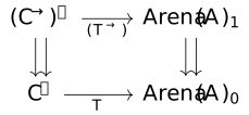
To construct the double category \mathsf {\mathbb Arena}(\mathcal {A}) of charts and lenses for an ordinary fibration \mathcal {A} \to \mathcal {C}, one can use the following procedure:
Form the square double category \mathcal {A}^\to \rightrightarrows \mathcal {A}
Take the fiberwise opposite of these objects: (\mathcal {A}^\to )^\mathrm {fop} \rightrightarrows \mathcal {A}^\mathrm {fop}.
Observe that fiberwise opposite preserves pullbacks, and hence this is again a double category.
Here we used the following result: If \mathcal {D} \to \mathcal {C} is a Grothendieck fibration and \mathcal {A} is any category, then \mathcal {D}^\mathcal {A} \to \mathcal {C}^\mathcal {A} is again a fibration (which classifies the lax limits of the composite \mathcal {A}^\mathrm {op} \to \mathcal {C}^\mathrm {op} \to \mathsf {Cat}), and a natural transformation is Cartesian iff it is levelwise Cartesian. It would be neat to obtain a similar result for Markov fibrations.
The first problem with this is that \mathcal {C}^\mathcal {A} does not generally inherit a Markov structure from \mathcal {C}. As we noted when we introduced diagram Markov categories, one has to consider the category \mathsf {Fun}(\mathcal {A},\mathcal {C}) of deterministic diagrams instead.
First, we will see that this indeed works for Markov prefibrations. This implies that (-)^\mathcal {A} lifts from fibrations to stochastic modules.
Let \mathcal {D} \to \mathcal {C} be a Markov prefibration. Recall that by \mathcal {C}^\to we denote the category of deterministic arrows in \mathcal {C}. Let \mathsf {Ar}(\mathcal {C}) denote the ordinary arrow category. Let now \mathcal {D}^\to denote the category \mathsf {Ar}(\mathcal {D}) \times _{\mathsf {Ar}(\mathcal {C})} \mathcal {C}^\to consisting of those arrows in \mathcal {D} which lie over a deterministic base (but again, where the morphisms consist of commutative squares whose other sides do not necessarily have deterministic bases). Then \mathcal {D}^\to \to \mathcal {C}^\to is a Markov prefibration.
This yields a functor \mathsf {MarkPreFib}(\mathcal {C}) \to \mathsf {MarkPreFib}(\mathcal {C}^\to ), so that (\mathcal {D}^\to )|_\mathrm {det} = (\mathcal {D}|_\mathrm {det})^\to . This equation induces a natural transformation \overline {(\mathcal {D}_0^\to )}|_\mathrm {det} \to (\overline {\mathcal {D}_0}|_\mathrm {det})^\to , which in turns gives a lift of (-)^\to to the category of stochastic module fibrations, where the induced algebra structure acts pointwise.
Noting that \mathcal {C}^\to is a Markov category with the "pointwise" structure, and the deterministic maps consist precisely of the pointwise deterministic maps, clearly \mathcal {D}^\to |_\mathrm {det} = \mathcal {D}|_\mathrm {det}^\to , and fibrations are stable under the formation of arrow categories, with Cartesian maps formed pointwise.
It is not trivial that this is a prefibration, because given a triangle in \mathcal {C}_\mathrm {det}^\to ---a "prism"---and a Cartesian lifting, we only know that the maps "at the ends" are Cartesian, not the maps between the triangles.
Therefore we can not immediately apply the unique lifting property to say that the square between the induced lifts \bar {Y_i}_{X_i} \to \bar {Y_i}_{Z_i} commute, given some map \bar {Y}_0 \to \bar {Y}_1 over Y_0 \to Y_1. However, by taking the pullback on both sides (and noting that pullbacks are functorial,) we can factor this square into two which live entirely over a deterministic base, and where the Cartesian property therefore imply commutativity.
We have already argued that this commutes with restriction to the deterministic part. The natural transformation is induced for completely abstract reasons, by applying (-)^\to to the unit to obtain a map \mathcal {D}_0^\to \to (\overline {\mathcal {D}_0}|_\mathrm {det})^\to = (\overline {\mathcal {D}_0}^\to )|_\mathrm {det}, which by the universal property of \overline {(-)} induces the desired map \overline {(\mathcal {D}_0^\to )}|_\mathrm {det} \to (\overline {\mathcal {D}_0}|_\mathrm {det})^\to .
Let \mathcal {A} be a small category, and let \mathcal {D} \to \mathcal {C} be a Markov prefibration. Let \mathsf {Fun}(\mathcal {A},\mathcal {D}) := \mathcal {D}^\mathcal {A} \times _{\mathcal {C}^\mathcal {A}} \mathsf {Fun}(\mathcal {A},\mathcal {C}). Then the functor \mathsf {Fun}(\mathcal {A},\mathcal {D}) \to \mathsf {Fun}(\mathcal {A},\mathcal {C}) is a Markov prefibration.
Note that \mathsf {Fun}(\mathcal {A},\mathcal {D}) is a limit of the categories \mathcal {D}^\to and prefibrations are stable under these limits.
The question is now
If \mathcal {D} is a Markov fibration, we get a stochastic module structure on \mathcal {D}|_\mathrm {det}^\mathcal {A}---does it present a markov fibration?
There is an induced map \mathsf {SChart}(\mathsf {Fun}(\mathcal {A},\mathcal {D}|_\mathrm {det})) \to \mathsf {Fun}(\mathcal {A},\mathcal {D}) (where the latter is taken by convention to mean the full subcategory of functors whose image in \mathcal {C} consists of deterministic arrows). Is this an isomorphism? (If it is, clearly this implies point 1)
Unfortunately it's not clear that either of these are true---the surjectivity of \mathsf {SChart}(\mathcal {D}|_\mathrm {det}) \to \mathcal {D} cannot a priori be lifted to the arrow category. The issue is that, given a map in \mathcal {D}^\to consisting of, say \phi _0,\phi _1, it is not sufficient to find charts representing each of these---we must find a chart of squares representing the square. This is not guaranteed by the Markov fibration structure, and a similar issue comes into play for the equivalence witnesses.
We may attempt to ignore this issue and simply try to form a double category \mathsf {SLens}(\mathcal {D}^\to ) \rightrightarrows \mathsf {SLens}(\mathcal {D}), given a stochastic module \mathcal {D}, but here the problem is that \mathsf {SLens} does not commute with limits in general. Hence we can not easily define a composition on the 2-cells of lenses obtained this way.
There are various ways we might attempt to remedy this problem. One approach would be to formulate a behavioural notion of "commutativity" for squares of stochastic lenses and charts, but the problem with this is that it is not obvious whether this property is stable under composition.
The basic problem stems from the fact that chart equivalences have a "directed" nature, and given a morphism of precharts (M,\phi ) \to (N,\psi ) and an equivalence (N,\psi ) \leftarrow (N',\psi ') (for example given by a stochastic section N' \to N satisfying suitable conditions), there is not in general a way to lift this back into an equivalent (M',\phi ') with a map to N'.
This observation leads to the idea that we might define a double category of precharts which has the directed equivalences among its morphisms (going only in one direction). We will begin by constructing this double category.
Let \mathcal {D} \to \mathcal {C} be a (Grothendieck) fibration, and let \mathcal {C} \to \mathcal {C}' be a faithful, identity-on-objects functor. Suppose \mathcal {C} admits pullbacks, and given a pair of morphisms P \to X,Y \in \mathcal {C}' over Z, where P \to X is in \mathcal {C}, there is a unique common factorization P \to X \times _Z Y.
The double category \mathsf {\mathbb Span}_{\mathcal {C}'}(\mathcal {C}) has \mathcal {C} as the vertical category, spans X \leftarrow P \to Y in \mathcal {C} equipped with a section X \to P \in {\mathcal {C}'} as horizontal cells, and maps of spans which commute with the sections as 2-cells.
The double category \mathsf {\mathbb Span}_{\mathcal {C}'}(\mathcal {D} / \mathcal {C}) lying over \mathsf {\mathbb Span}_{\mathcal {C}'}(\mathcal {C}) has \mathcal {D} as the vertical category, and spans \bar {X} \xleftarrow {f} \bar {P} \xrightarrow {g} \bar {Y} where f is Cartesian, decorated with a section X \to P in \mathcal {C}' as the horizontal cells, and maps of such spans (so that the underlying thing commutes with the sections) as the 2-cells. We will call the horizontal cells decorated spans.
There is an apparent forgetful functor \mathsf {\mathbb Span}_{\mathcal {C}'}(\mathcal {D} / \mathcal {C}) \to \mathsf {\mathbb Span}_{\mathcal {C}'}(\mathcal {C})
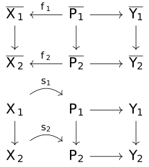
To spell it out, a 2-cell in \mathsf {\mathbb Span}_{\mathcal {C}'}(\mathcal {D} / \mathcal {C}) consists of a diagram of this form in \mathcal {D}, where f_1,f_2 are Cartesian,
and (writing X_1 for the object underlying \overline {X_1}, and so on) two sections s_1,s_2 of the underlying maps in \mathcal {C}', so that the second diagram also commutes in \mathcal {C}':
Naturally, we are interested in the case of \mathsf {\mathbb Span}_{\mathcal {C}}(\mathcal {D} / \mathcal {C}_\mathrm {det}) for a stochastic module \mathcal {D}. Then the decorated spans are representatives for stochastic charts. We will start by introducing a loosed notion of 2-cell for these spans, which combines the directed equivalences with the ordinary deterministic 2-cells of spans.
Let \mathcal {C} be a Markov category and let \mathcal {D} be a stochastic module over \mathcal {C}.
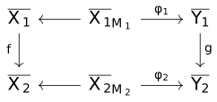
Let (M_1, \phi _1): \bar {X_1} \leftrightarrows \bar {Y_1}, (M_2, \phi _2): \bar {X_2} \leftrightarrows \bar {Y_2} be decorated spans in \mathsf {\mathbb Span}_{\mathcal {C}}(\mathcal {D} / \mathcal {C}_\mathrm {det}), and let f: \bar {X_1} \rightrightarrows \bar {X_2}, g: \bar {Y_1} \to \bar {Y_2} be morphisms in \mathcal {D}, so that we have a square
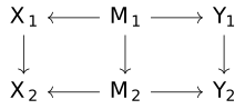
A 2-cell of decorated spans for this data consists of a morphism m: M_1 \to M_2 \in \mathcal {C} (that is, possibly stochastic), satisfying the following two conditions. First, the diagram
in the base must commute. Given this, there is an induced square
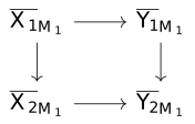
in \mathcal {D}_{M_1}, where the bottom map is given by pulling back \phi _2 along m, in the sense of Lemma [efr-VF6V]. The second condition is that this square must also commute.
2-cells of decorated spans compose---that is, given a diagram
where the horizontal maps are decorated spans, and the vertical maps are maps in \mathcal {D} with deterministic base, and given maps of decorated spans \phi _1 \xrightarrow {\alpha } \phi _2 \xrightarrow {\beta } \phi _3, there is a map of decorated spans \phi _1 \to \phi _3
We can easily compose the two maps to get M_1 \to M_3. Now, the question is whether the perimeter of this diagram commutes:
Note that the top square is commutative by assumption, since pullbacks compose (even along stochastic maps) and this is the assumption that \alpha is a cell. The bottom square is the result of pulling back a commutative square over M_2 again along \alpha . Note that pullback along stochastic morphisms is not in general functorial---but since the vertical parts of this square are themselves pulled back from X_2,Y_2, this composition is preserved by pullback along \alpha : M_1 \to M_2. This finishes the proof.
2-cells of decorated spans compose horizontally: Given a square
where the horizontal maps are precharts and the vertical maps are morphisms in \mathcal {D}|_\mathrm {det}, and given \alpha : \phi _1 \to \phi _2 and \beta : \psi _1 \to \psi _2, there is a prechart morphism \psi _1\phi _1 \to \psi _2\phi _2.
Unlike the proof of Lemma [efr-DRU6], this is straightforward: If the carrier of \phi _i is M_i, and of \psi _i,N_i (for i=1,2), then by definition the composites are carried by the pullback M_i \times _{Y_i} N_i. There is a canonical map M_1 \times _{Y_1} N_1 \to M_2 \times _{Y_2} N_2 over M_2, N_2, given by the independent pairing of \alpha and \beta .
Since pullbacks compose, the square over M_1 \times _{Y_1} N_1 that must commute is given by the two commutative squares induced by \alpha ,\beta , pulled back and composed with each other. Here we are pulling back along the deterministic projections from the pullback, and hence these commutative squares are preserved, and hence the composite square commutes as well.
Let \mathcal {D} be a stochastic module over \mathcal {C}. There is a double category \widetilde {\mathsf {\mathbb Span}}(\mathcal {D})^\mathrm {chart} which has decorated spans as its horizontal maps, morphisms in \mathcal {D}|_\mathrm {det} as its vertical maps, and decorated span 2-cells as its 2-cells.
Moreover, there is another double category \widetilde {\mathsf {\mathbb Span}}(\mathcal {D})^\mathrm {lens} which has decorated spans in \mathcal {D}^\mathrm {fop} as its horizontal maps instead.
(The modification of everything above to lenses instead of charts is obvious).
In fact, the globular 2-cells are in a sense exactly the equations defining the set of charts:
Suppose given a square
in \widetilde {\mathsf {\mathbb Span}}(\mathcal {D})^\mathrm {lens} (or \widetilde {\mathsf {\mathbb Span}}(\mathcal {D})^\mathrm {chart}) Suppose further the underlying square in \mathcal {C} is deterministic. Then:
If there exists a filling decorated span 2-cell, the image in \mathsf {\mathbb Arena}(\mathcal {D}|_\mathrm {det}) commutes.
If M_1 is the carrier of \phi _1 and the left leg M_1 \to X_1 is an isomorphism, then this implication is an equivalence.
Given a stochastic chart carried by X \leftarrow M \to Y, so that X \to Y is deterministic, recall that we can first pull back to the equalizer M' \hookrightarrow M of the two maps M \to X \to Y, M \to Y, then along the prescribed section X \to M'. Note that this gives a 2-cell from this canonical representative with carrier X to the initial representative.
Given two such cells, we get a square
But as part of the square surrounding the 2-cell, there is given a map X_1 \to X_2, which must make this square commute. The functoriality of base change (pulling back the map \phi _2) proves this bottom map is again a 2-cell.
But the property for this map to be a 2-cell is exactly the property for this square to be a commutative square in \mathsf {\mathbb Arena}{\mathcal {D}|_\mathrm {det}}. This proves both parts of the statement.
Double Categories of Stochastic Dynamical System[efr-7DV5]
A stochastic dynamical systems theory consists of a stochastic module \mathcal {D} over \mathcal {C} equipped with a section T: \mathcal {C}_\mathrm {det} \to \mathcal {D}|_\mathrm {det} of the underlying fibration.
We adopt the notation \widetilde {\mathsf {\mathbb Arena}}(\mathcal {D}) for the double category which was denoted \widetilde {\mathsf {\mathbb Span}}(\mathcal {D})^\mathrm {lens} above. We use the symbol \leftrightarrows for the horizontal (span) morphisms and \rightrightarrows for the vertical morphisms (in \mathcal {D}).
Given a stochastic dynamical systems theory (\mathcal {D}, T), the double category of dynamical systems\mathsf {Sys}(\mathcal {D},T) has
Horizontal morphisms given by a pair f: S \to S', g: \bar {A} \rightrightarrows \bar {B} \in \mathcal {D}, c where c is a square filling \xi , \xi ', Tf, g
Vertical morphisms given by a pair f: S \to S', g: \bar {A} \leftrightarrows \bar {B} \in \overline {\mathcal {D}}, c where c is a square filling Tf, g \xi , \xi ', 1_{\bar {B}}
Let T,\mathcal {D} be a stochastic dynamical systems theory.
Then T,\mathcal {D}|_\mathrm {det} is an ordinary dynamical systems theory.
There is a double functor \mathsf {Sys}(T,\mathcal {D}|_\mathrm {det}) \to \mathsf {Sys}(T,\mathcal {C}). This functor is full on vertical morphisms, and on 2-cells.
Let \mathsf {Sys}(T,\mathcal {D})_\mathrm {det} denote the subcategory spanned by systems with deterministic readout, prelenses with deterministic base, and all the morphisms of \mathcal {D}. Then the restricted functor \mathsf {Sys}(T,\mathcal {D}|_\mathrm {det}) \to \mathsf {Sys}(T,\mathcal {D})_\mathrm {det} admits a chartwise right adjoint, which assigns to each system or prelens its equivalence class.
The functor simply acts as the functor in Proposition [efr-JQI9]. Since that inclusion is full on 2-cells, this one is full on vertical morphisms, and since a 2-cell in \mathsf {Sys} is merely a 2-cell in \mathsf {\mathbb Arena} between specific objects, it is also full on 2-cells.
The right adjoint property likewise follows from the analogous property of the inclusion functor on arenas.
Let \mathcal {D} be a Markov prefibration. Then there is a double functor \mathsf {\mathbb Arena}(\mathcal {D}|_\mathrm {det}) \to \widetilde {\mathsf {\mathbb Arena}}(\mathcal {D}), which acts as identity on the morphisms of \mathcal {D}, and carries each lens (f: X \to Y, \phi : f^*\bar {Y} \to \bar {X}) to the prelens (X \leftarrow X \to Y, \phi ). This double functor is full on 2-cells.
The restriction to \mathsf {\mathbb Arena}(\mathcal {D}|_\mathrm {det}) \to \mathsf {\mathbb Arena}(\mathcal {D})_\mathrm {det} admits a right adjoint, which carries every prelens to its equivalence class.
First we must verify functoriality with respect to lens composition. To that end, let X \xrightarrow {f} Y \xrightarrow {g} Z be deterministic morphisms and \phi ,\psi be lenses over them.
Their composite as prelenses has carrier X \times _Y Y = X and f^*(\psi )\phi as the morphism in the fiber, which is exactly the prelens associated to their composite as lenses.
Second, we must verify fullness on 2-cells. But this is a special case of Proposition [efr-10CM].
Finally, Proposition [efr-10CM] is precisely the statement that assigning a prelens to its equivalence class lens is right adjoint to this (and in particular that it forms a functor)
Recall that in Myers' categorical dynamical systems theory, trajectories of a system \xi : TS \leftrightarrows \bar {A} are identified with chart morphisms from a "clock" system---thus for example trajectories of a smooth dynamical system M \to TM are exactly those maps \gamma : \mathbb {R} \to M which, when \mathbb {R} is equipped with the vectorfield dx/dt = 1, are homomorphisms.
In general this presents an issue for our replacement category \mathsf {Sys}(T,\mathcal {D})---since we wish to regard two systems given by equivalent lenses as equivalent, but their set of homomorphisms from a given clock system is not necessarily in bijection. In the general case, we do not presently have a way around this problem---but at least for clock systems with deterministic readout, the above presents a solution: choosing the initial representative for such a system, we find that the set of trajectories does not depend on the equivalence class of the target system.
The triple category of dynamical systems[efr-MWCE]
Let \mathcal {A} \to \mathcal {C}, T: \mathcal {C} \to \mathcal {A} be a symmetric monoidal dynamical systems theory. Then this diagram:
depicts two strict double categories, each with a symmetric monoidal structure, and a strict double functor between them which is (non-strictly) a symmetric monoidal functor. This induces an object of \mathsf {SymMon}(\mathsf {Act}(\mathsf {DblCat})). Applying \mathsf {\mathbb Para}(-) under \mathsf {SymMon}(-), we obtain a symmetric pseudomonoid in internal pseudocategories in \mathsf {DblCat}. Denote by \mathsf {BiSys}(\mathcal {C},\mathcal {A},T) this induced object.
\mathsf {BiSys}(\mathcal {C},\mathcal {A},T) has the following structure: The objects are simply the objects of \mathcal {A}---the bundles.
There are three types of 1-cell: Lenses, that is morphism in \mathcal {A}^\mathrm {fop}, which we write A \leftrightarrows B, charts, that is morphisms in \mathcal {A}, which we write A \rightrightarrows B, and bisystems, which are pairs (S \in \mathcal {C}, TS \otimes A \leftrightarrows B), and which we write A \nrightarrow B.
Moreover there are three types of 2-cell:
Lens-chart cells, which are the 2-cells of \mathsf {\mathbb Arena}(\mathcal {A}). Note that this double category is thin. We will say a square of lenses and charts commutes if it is filled by such a 2-cell.
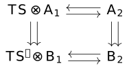
Chart-bisystem cells---given charts A_1 \rightrightarrows B_1, A_2 \rightrightarrows B_2 and systems TS \otimes A_1 \leftrightarrows A_2, TS' \otimes A_2 \leftrightarrows B_2, a square filling this is a choice of map S \to S' \in \mathcal {C} so that the resulting lens-chart square
commutes.
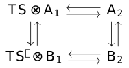
Lens-bisystem cells. Given lenses A_1 \leftrightarrows B_1, A_2 \leftrightarrows B_2, and systems TS' \otimes A_1 \leftrightarrows A_2, TS' \otimes B_1 \leftrightarrows B_2, a 2-cell consists of an isomorphism S' \xrightarrow {\sim } S' so that the resulting square of lenses commutes (recall that isomorphism charts are the same as isomorphism lenses).
The charts, bisystems and chart-bisystem cells form a pseudo double category with the obvious composition. So do the lenses, bisystems and lens-bisystem cells. Finally, there is a notion of 3-cell given by a box whose sides are 2-cells of each kind, so that the resulting diagram in \mathcal {C} (with isomorphisms on two sides) commutes.
The lens-bisystem double category is \mathsf {\mathbb Para}_{\mathcal {C}^\simeq }(\mathsf {\mathbb Arena}{\mathcal {A}}_0) (recall that \mathsf {\mathbb Arena}{\mathcal {A}}_0 = \mathcal {A}^\mathrm {fop}), with the action given by the functor T (restricted to isomorphisms). The chart-bisystem double category is the result of taking \mathsf {BiSys}(\mathcal {C},\mathcal {A},T), a pseudocategory in double categories, and applying \mathsf {PsCat}((-)_h) : \mathsf {PsCat}(\mathsf {DblCat}) \to \mathsf {PsCat}(\mathsf {Cat}) where (-)_h takes the horizontal category of a (strict) double category.
The 3-cells, of course, are the 2-cells of \mathsf {\mathbb Para}_{(\mathcal {C}^\to )^\simeq }(\mathsf {\mathbb Arena}(\mathcal {A})_1). Analogously to the above, for each class of 1-cells, there is a
double category with those as the objects, the two types of cell as the two morphisms, and the 3-cells as the 2-cells.
All of these six double categories admit a symmetric monoidal structure.
We can recover the ordinary category of (Moore) systems as the slice over I, in the following sense:
In a double category \mathbb {C}, there is a "horizontal slice" 1-category having objects the horizontal maps A \to B and morphisms given by 2-cells that are identity on the left boundary, composed vertically. Similarly there is a "vertical slice". This is given by a similar pullback in \mathsf {Cat}---we simply do this one level up.
Note that Myers' construction of the double fibration \mathsf {Sys}(\mathcal {C},\mathcal {A},T) \to \mathsf {\mathbb Arena}{\mathsf {Cat}} in fact uses the vertical slice in this sense.
This somewhat trivial observation means that any composition in \mathsf {BiSys}(\mathcal {C},\mathcal {A},T) which produces 2-cell under I in fact produces a morphism of systems in the ordinary sense. Replacing I with another object, we may regard the slices as further-parametrized versions of \mathsf {Sys}(\mathcal {C},\mathcal {A},T).
There is essentially no difficulty in applying this to the Markov case:
Let (\mathcal {C}, \mathcal {A}, T) be a stochastic dynamical systems theory. Consider the double category whose vertical category is \mathcal {C}_\mathrm {det} and horizontal category is \mathcal {C}, with commutative squares as the 2-cells (this is the transpose of \mathcal {C}^\to \rightrightarrows \mathcal {C}). This carries an obvious symmetric monoidal structure, and acts on the double category of stochastic arenas \widetilde {\mathsf {\mathbb Arena}}(\mathcal {A}) via the functor T. Denote by \mathsf {BiSys}^M(\mathcal {C},\mathcal {A},T) the symmetric monoidal triple category induced as in Definition [efr-EPI9] by this data.
The information contained in \mathsf {BiSys}^M(\mathcal {C},\mathcal {A},T) is much as above, although the complications involved in the double category of stochastic arenas remain present.
Our bisystems are reminiscent of the energy-driven systems of Capucci, Lynch, and Spivak (Reference [energy-driven-systems]). Indeed, their \mathbb {C} \mathsf {org} is essentially the bisystems in the (ordinary) doctrine of smooth dynamical systems. As we mentioned in the introduction, Shapiro and Spivak (Reference [shapiro-spivak-dynamic-operads]) have previous developed a structure \mathbb {O} \mathsf {rg} which consists of the bisystems for the discrete dynamical systems doctrine (i.e \mathsf {Set}^\to \to \mathsf {Set}). \mathbb {O} \mathsf {rg} has a tremendous amount of structure coming from the representation of lenses in this doctrine as the category of polynomial functors, which can't be replicated for a general systems theory (and certainly not for a general stochastic systems theory).
A Stochastic Dynamical Systems Theory of Smooth Manifolds[efr-9J8G]
In this section, as the title suggests, we construct a stochastic dynamical systems theory of smooth manifolds, with the usual tangent bundle.
The main point is to construct a Markov category containing the smooth manifolds which is pullback-positive. We do this by considering the larger category of diffeological spaces. In order to make the topology work, we need to complicate the notion of diffeological space a bit, but having done so, we obtain a representable Markov category which is pullback-positive, and contains \mathsf {SmMfd} as a full subcategory of the deterministic maps. A kernel p: M \to N is a Markov kernel valued in Radon measures which is weakly continuous---so induces a linear map C(N) \to C(M) taking \phi to the function x \mapsto E_{p_x}\phi on the spaces of continuous functions---and which furthermore smooth in the sense that this operation preserves the smooth functions.
This Markov category of "smooth stochastic maps" may be of some independent interest.
Let \mathsf {CartSp} denote the full subcategory of \mathsf {SmMfd} spanned by the objects \mathbb {R}^n for each n. Note that \mathsf {CartSp} has finite products, and is generated by the object \mathbb {R} under finite products.
A smooth space is a sheaf on \mathsf {SmMfd} in the standard topology of open covers.
A smooth space X is a diffeological space if, for each M \in \mathsf {SmMfd}, the map X(M) \to \prod _{p \in M} X(\{p\}) is injective.
A diffeological space with underlying set X is called a diffeology on X, and consists of specifying which maps \mathbb {R}^n \to X are smooth. We call these maps smooth plots.
Given a subset X' \subset X, there is an obvious canonical diffeology on X' given by taking the plots to be those functions whose image in X is smooth. We call this the subspace diffeology.
A morphism of diffeological spaces is called a smooth map. It is equivalently a function X \to Y which carries smooth plots to smooth plots.
A diffeo-topological space is a diffeological space X equipped with a topology \tau so that all the smooth plots are continuous.
A map of diffeo-topological spaces is a smooth map (for the diffeology) which is also continuous (for the topology).
Given a subset X' \subset X, there is an obvious canonical diffeo-topology on X' given by taking the plots to be those functions whose image in X is smooth, and equipping X' with the subspace topology.
The category of diffeo-topological spaces admits all limits, given by taking the limits in topological spaces and diffeological spaces (which have the same underlying set).
Let X be a diffeo-topological space whose underlying space is Tychonoff. Then the space of probability measures P(X) has a canonical diffeology given by those plots f: U \to P(X) so that for each continuous function g on X, the resulting map u \mapsto E_{f(u)g} is continuous, and if g is smooth, then this is smooth as well. With this diffeology, and the topology of weak convergence, P(X) is a diffeo-topological space. This defines a commutative affine monad on \mathsf {TychDiff}, the category of such diffeo-topological spaces.
The topology of weak convergence on P(X) is such that A \to P(X) is continuous if and only if the expectation map carries continuous functions to continuous functions. But this is part of the requirement to be a smooth plot, so certainly this is a diffeo-topological space.
Since the linear operator associated to x \in X under the unit X \to P(X) is merely evaluation at x, the unit is clearly smooth.
Consider \mu : PPX \to PX. To test this is smooth, let f: U \to PP(X) be a plot. We must show \mu f is a plot. So let v: X \to \mathbb {R} be a continuous (resp. smooth) function. We must show its expectation a is continuous (resp. smooth) function of u \in U.
By construction E(v) : PX \to \mathbb {R} is continuous (resp. smooth), and so since f is a plot, the map u \mapsto E_{f(u)}E(v) is continuous (resp. smooth). But this is exactly what we wanted.
The monad laws follow from their holding in \mathsf {Tych}. Since a commutative monad is equivalently a strong monad satisfying a certain equation (which holds for this monad in \mathsf {Tych} and therefore also here), it suffices to show that the strength P(X) \times Y \to P(X \times Y) is smooth. This follows by a completely analogous argument.
The category \mathsf {TychDiffStoch} of Tychonoff diffeological spaces and Kleisli maps for the monad P described in Proposition [efr-7RS2] is a pullback-positive Markov category. Its deterministic category is \mathsf {TychDiff}. There is a fully faithful functor \mathsf {SmMfd} \to \mathsf {TychDiff} which preserves transverse pullbacks.
The maps between smooth manifolds are given by weakly continuous families of Radon probability measures, so that the expectation operator carries smooth maps to smooth maps.
Since we describe properties of kernels in terms of their corresponding linear operator on function spaces, it would seem natural to take the function spaces as the basic object. Hence we might consider the category C^\infty -algebras with some relaxed notion of maps between them. The tricky part there is to find some reasonable class of maps so that the tensor product (coproduct) of C^\infty -algebras extends to these. (Since it is not the same as the tensor product of \mathbb {R}-algebras, linear maps do not automatically extend to the tensor product). In particular, when considering kernels *_1 \to X where *_1 is a "fat point of order 1"---that is, functions on 1_* have a value at the point and a derivative---it is not clear what sort of continuity condition the derivative operation on C^\infty (X) should satisfy, nor how to define this in a general way for all C^\infty -algebras. It would certainly be of interest to synthetic computational geometry to have such a Markov category, but we leave this for future work.
We will now give an example of how to represent the training dynamics of a machine learning system using the tools developed so far.
As discussed previously, given a parameterized function F: P \times X \to Y, its reverse derivative naturally becomes a parameterized lens, and the composition of these describe how gradient vectors are passed around to compute an update during training. It is natural to want to compose this lens with the data-generating distribution I \to X \otimes Y, (along with some more context describing the loss function, etc) to obtain the training dynamics of such a model. This requires a category of parameterized lenses which allows stochastic maps in the base. The goal of combining this feature with non-trivial tangent bundles was one of the original motivations for developing a theory of stochastic lenses.
Consider the Markov prefibration \mathsf {TychDiffStoch}^\to \to \mathsf {TychDiffStoch}. Equip this with the section T(X) = X \otimes X \xrightarrow {\pi _0} X - this described discrete-time systems (whose update is required to be smooth in the input and present state). This is clearly a symmetric monoidal functor and thus defines a systems theory. Note that this is completely different from the ordinary tangent bundle, despite the coincidence of notation.
Let m_1: TS_2 \otimes X_1 \leftrightarrows Y_1 and m_2: TS_2 \otimes X_2 \leftrightarrows Y_2 be two bisystems in this theory.
As in § [efr-SREZ], we may define a parameterized lens (TS_1 \& TS_2) \otimes (X_1 \oplus X_2) \leftrightarrows (Y_1 \oplus X_2), denoting by \oplus the coproduct in lenses, and by \& the Markov structure defined in Corollary [efr-FT8J]. Observe that TS_1 \& TS_2 is simply the indexed set (S_1 \coprod S_2) \otimes S_1 \otimes S_2 \to S_1\otimes S_2. There is an obvious indexed map from this to T(S_1 \otimes S_2) = S_1 \otimes S_2 \otimes S_1 \otimes S_2, given by (\operatorname {inl} s_1', s_1,s_2) \mapsto (s_1', s_2, s_1, s_2) and (\operatorname {inr} s_2', s_1, s_2) \mapsto (s_1,s_2',s_1,s_2). In words, we receive an update either to the S-state or to the S'-state. We apply this update to the relevant state and leave the other alone. This defines a lens T(S_1 \otimes S_2) \leftrightarrows T(S_1) \& T(S_2), which we may compose with the above to obtain a bisystem T(S_1 \otimes S_2) \otimes (X_1 \oplus X_2) \leftrightarrows Y_1 \oplus Y_2. Let us denote this by m_1 \oplus m_2.
This has very much the same flavor as the external choice for open games, although we will not develop the theory of this operation in detail here.
Now, given a smooth (deterministic) map F: P \times X \to Y, where P,X,Y are smooth manifolds (not merely diffeo-toplogical spaces), we obtain a lens T^*(F): {T^*P \choose P} \otimes {T^*X \choose X} \leftrightarrows {T^*Y \choose Y}, where T^*(-) denotes the cotangent bundle. (This does not, prima facie, make sense for a general diffeo-topological space).
Let us take as given some family of lenses T(S) = {S \otimes S \choose S} \leftrightarrows {T^*S \choose S} for various S. Such an operation amounts to choosing a way of updating s \in S given a cotangent vector---hence we can see it as an optimization algorithm. One example of such would be gradient descent, which given a choice of Riemann structure on S, takes a step of a given length in the direction which most quickly decreases the given covector.
(It should be noted that there are more complicated optimization strategies which don't fit this particular pattern - for example, momentum algorithms have to maintain some extra internal state other than s \in S. But let's stick with this pattern for this example). Note also that we're not assuming the optimizers are a natural transformation or anything like that.
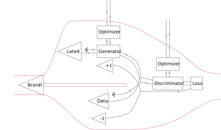
Now we are ready to build the neural network architecture known as a generative adversarial network, or GAN (Reference [gan-paper]). Let us first describe the idea. Our goal is to generate additional samples from some distribution, given a set of existing samples---for example, our goal may be to generate more pictures in the same style as an existing corpus. Suppose our data is of type X, and let d: I \to X be the data distribution. We fix some latent distribution\lambda : I \to L, where L is any space of our choice---usually, L is \mathbb {R}^n and \lambda is a Gaussian. Finally we choose two neural networks, the generatorG: P_G \otimes L \to X, and the discriminatorD: P_D \otimes X \to \mathbb {R}. The goal of the discriminator is to discriminate real samples from the data from generated samples, by providing a low value on the generated samples and a high value on the true samples.
The training process now goes as follows: for each step of training, we either sample from the latent distribution, and have the generator use this to generate a sample, or draw a sample from the data distribution (choosing between these with some probability p). Then in either case, we have the discriminator score the generated sample. If the sample was generated by the generator, the discriminator's loss is equal to its output, otherwise it is equal to -1 times its output. We update the discriminator according to the gradient of this loss (minimizing it), and update the generator (if we are in the branch where it was run) according to the negative of the gradient of this loss with respect to the generator parameters---this amounts to doing a gradient descent update on the generator for the negative of the discriminator loss.
The two "tapes" branching off at the start represent two maps (bisystems) composed by \oplus , while the backwards wires indicate the flow of the gradients. The ground symbol indicates a value being discarded. Note that the theory of tape diagrams has only been developed formally for distributive categories, and for essentilly the same reason as in § [efr-SREZ], we do not have distributivity in this case. However, the interpretation of this diagram is still unambiguous---distributivity is required to make tape diagrams complete, not to make them sound. Concretely, if we tried to represent the tensoring of this system with another system, we would have no way of doing it, but if the category was distributive we could do so by adding this additional system to each of the branches. Still, the figure is best viewed as a visual aid rather than a formal representation.