The Universal Property of Measure-Theoretic Probability › Preliminaries [efr-8P2U]
The Universal Property of Measure-Theoretic Probability › Preliminaries [efr-8P2U]
The terminology Markov category was introduced by Fritz in Reference [fritz-synthetic-markov-cats], although the idea goes back to the work of Golubtsov, Reference [golubtsov-kleisli]. They have been developed extensively as an abstract foundation for probability theory, see eg Reference [fritz-gonda-perrone-rischel-rep], Reference [rischel-fritz-infinite-products], Reference [law-large-nums-fritz-etal], Reference [fritz-gonda-perrone-2021]. We now review the basics.
There is a strictification result (Reference [fritz-synthetic-markov-cats], Theorem 10.17) for Markov categories which allows us to freely elide the structural isomorphisms—we generally do so throughout this paper.
The morphisms of a Markov category are thought of as probability kernels, that is functions with values in probability measures (where these terms may be interpreted in a suitably abstract sense). The copy and delete maps are the non-stochastic maps which either copy or delete their input.
It is simple to verify that every Markov category is semiCartesian, and thus the only choice involved in equipping a symmetric monoidal category with a Markov structure is \mathrm {copy}_X. A morphism f :X \to Y \in \mathcal {C} is called deterministic if it is a homomorphism for the given comonoid structure. The subcategory of deterministic morphisms is denoted \mathcal {C}_\mathrm {det} \subseteq \mathcal {C}. It is always a symmetric monoidal subcategory, and Cartesian. Conversely, every Cartesian category carries a unique Markov structure.
We will often use the notation of Cartesian categories and denote by \pi _A the map (A \otimes \mathrm {del}_B): A \otimes B \to A.
Given two maps f: X \to A, g: X \to B, there is a distinguished pairing X \to A \otimes B, given by (f \otimes g)\mathrm {copy}_X. This is called the independent pairing of f and g. Note that by naturality of \mathrm {del} and the comonoid equations, f and g can be recovered from this pairing by postcomposing with \pi _A or \pi _B. Thus "being independent" is a property of kernels with a tensor product as its codomain. We generalize this to higher tensor products in the obvious way.
The following class of examples captures almost all Markov categories of interest.
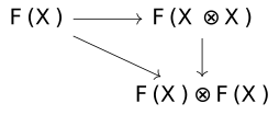
The undecorated term Markov functor was defined in Reference [fritz-synthetic-markov-cats] to mean what we above called a strong Markov functor. From this point, "Markov functor" will always mean the strong notion.
Our goal in this paper is to construct certain functors between Markov categories. The following lemma is helpful in this regard.
We denote by \mathsf {BorelStoch} the category of standard Borel spaces and Markov kernels (Reference [fritz-synthetic-markov-cats], Section 4). We denote by \mathsf {Borel} the category of standard Borel spaces and measurable maps. Note that \mathsf {Borel} = \mathsf {BorelStoch}_\mathrm {det}. Recall that the standard Borel spaces are those measurable spaces arising as the Borel \sigma -algebra on Polish spaces. By Kuratowski's theorem these are either discrete on a countable set, or isomorphic to the real numbers (in the Borel \sigma -algebra). Recall also that \mathsf {BorelStoch} is the Kleisli category of a monad on \mathsf {Borel} called the Giry monad, see Reference [giry-1982] (see also Reference [fritz-synthetic-markov-cats] section 4 for a review of the history of this concept).
The categorical notion of product extends obviously to define infinite products. Infinite products exist in many Markov categories of interest, such as those of measurable spaces and Markov kernels, but they clearly can't be characterized by their usual universal property. Instead, we can ask them to be Kolmogorov products, in the following sense:
These were introduced in Reference [rischel-fritz-infinite-products], where it was also shown that \mathsf {BorelStoch} admits countable Kolmogorov products (Example 3.6).
Note that given any Markov functor F: \mathcal {C} \to \mathcal {D}, and a family X_j so that the Kolmogorov product \bigotimes _j X_j exists, there is a family of (necessarily deterministic) maps F(\bigotimes _j X_j) \to \bigotimes _{j \in F} X_j for every finite F \subset J. As usual we say F preserves Kolmogorov products if this collection exhibits F(\bigotimes _j X_j) as the Kolmogorov product of the family F(X_j). If \mathcal {C}, \mathcal {D} admit Kolmogorov products of a given cardinality, F preserves them if and only if F_\mathrm {det} : \mathcal {C}_\mathrm {det} \to \mathcal {D}_\mathrm {det} preserves products of this cardinality.
When the family X is constant, we will denote the Kolmogorov product \bigotimes _{i \in J} X simply by X^J.
If \bigotimes _{i \in J} X_i is a Kolmogorov product and f_i: A \to X_i is a collection of kernels, there is a canonical independent coupling (f_i): A \to \bigotimes _i X_i, given as the limit of the finite independent couplings A \to \bigotimes _{i \in F} X_i. In the case where all f_i (and all the X_i) are equal, we will denote this simply as f^J : A \to X^J.
The Kolmogorov product (I + I)^\omega = 2^\omega will play an important role in this paper. We generally write 0,1 : I \to 2 for the two canonical points in 2. If b \in 2^\omega is an element, 0.b, 1.b, 001101.b \in 2^\omega denote the result of prepending the given string to b. We may also write 0.2^\omega instead of \{0\} \otimes 2^\omega for the subobject given by those streams starting with a 0, and so on.