Thesis Cutting Board [efr-003Z]
- November 19, 2024
-
Eigil Fjeldgren Rischel
Thesis Cutting Board [efr-003Z]
- November 19, 2024
- Eigil Fjeldgren Rischel
Bidirectionality in graphical models [efr-0002]
- May 25, 2024
-
Eigil Fjeldgren Rischel
Bidirectionality in graphical models [efr-0002]
- May 25, 2024
- Eigil Fjeldgren Rischel
Definition Structural Causal Model [efr-0003]
- May 25, 2024
-
Eigil Fjeldgren Rischel
Definition Structural Causal Model [efr-0003]
- May 25, 2024
- Eigil Fjeldgren Rischel
Let G be a (finite) directed acyclic graph (DAG). Then a structural causal model (SCM) on G consists of
- For each vertex v \in V(G), measurable spaces \mathcal {X}_v, \mathcal {E}_v
- A family of independent random variables E_v \in \mathcal {E}_v---these are called the exogenous variables
- For each v, a measurable function \phi _v: \mathcal {E}_v \times \prod _{v' \to v} \mathcal {X}_{v'} \to \mathcal {X}_v (note that if v has no parents, the product is just a singleton)
There is a significant existing literature (see Abstracting causal models, Reference [rischel_compositional_2021], Reference [rubenstein_causal_2017]. For a survey see Reference [zennaro_abstraction_2022]) studying transformations between structural causal models. These have generally been called something like abstractions, the typical examples being the relationship between a high-level and a low-level model of the same system. However, the precise properties that we should ask for in such a transformation have turned out to be somewhat subtle. The most obvious condition to impose is to ask, for any possible variable we could intervene on, say X, and any other variable (or collection of variables) Y, that the diagram
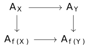
The main problem with this condition is that it is simply too strict. We generally can't ask that every low-level intervention is well-modeled by the corresponding high-level intervention. Rather, each high-level intervention corresponds to some distribution of the corresponding low-level variables, and we must ask that a diagram of this form:
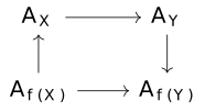
The key here is that control information flows in the opposite direction from measurement information. This phenomenon repeats in many examples.
Bidirectionality for control [efr-0004]
- May 25, 2024
-
Eigil Fjeldgren Rischel
Bidirectionality for control [efr-0004]
- May 25, 2024
- Eigil Fjeldgren Rischel
Consider a discrete-time, continuous-space, controlled, nonlinear dynamical system with noise. By this, I mean some transition function F(x,u): \mathbb {R}^n \times \mathbb {R}^p \to \mathbb {R}^n, along with a given "noise distribution" \mu on \mathbb {R}^n. The intended meaning is that x_{n+1} = F(x_n,u_n) + v_n, where u_n \in \mathbb {R}^p is a variable which can be controlled (depending on x_1, \dots x_n,) and (v_n)_{n=0,\dots } is a sequence of iid random variables distributed according to \mu (for simplicity, we assume everything is time-invariant). Without any assumptions of linearity or the like on F, it is hard to apply traditional control methods. Therefore we'd like to partition \mathbb {R}^n into a discrete set of components, and apply reinforcement learning algorithms to the resulting dynamics (or just straightforward dynamical programming, depending on the situation).
Suppose we have such a partition p: \mathbb {R}^n \to I, with I some discrete index set. We want to build some sort of controlled dynamical system on I (really a Markov Decision Problem). A priori, however, it seems the probability of being able to transition from i to j is highly dependent on where in p^{-1}(i) we are.
The trick to building an MDP is to choose u(x,i), where x is our current state and i is the target region, in such a way that x^i := F(x,u(x,i)) does not depend on x---then the distribution on the next state is just the distribution of p(x^i + v_n), which can be determined ahead of time for each i. i \mapsto x^i is a section of p---this bidirectionality is completely analogous to what we saw for abstractions between graphical models.
The datum u(-,=): \mathbb {R}^n \times I \to \mathbb {R}^p is the backwards part of a lens \binom {\mathbb {R}^p}{\mathbb {R}^n} \to \binom {I}{I}. Actually, this raises a subtlety we swept under the rug above---it may not be possible to find u(x,i) satisfying F(x,u(x,i)) = x_i for all pairs x,i. Hence we need to restrict ourselves to those where it is possible---and because we're trying to abstract away x, we need to consider those i so that it's possible for all x in our current component. This will bring us to consider dependent lenses.
Composition with graded predicates [efr-0009]
- June 5, 2024
-
Eigil Fjeldgren Rischel
Composition with graded predicates [efr-0009]
- June 5, 2024
- Eigil Fjeldgren Rischel
Suppose T: X \to \Delta (Y) is a stochastic map, and suppose \phi ^\epsilon is a graded predicate on Y (in particular, \phi ^\epsilon (y) \Rightarrow \phi ^{\epsilon '}(y) if \epsilon < \epsilon ').
Then we can define T^{-1}(\phi )^\epsilon , a graded predicate on X, by T^{-1}(\phi )^\epsilon (x) if there exists \epsilon _1 + \epsilon _2 = \epsilon with P(\phi ^{\epsilon _1}(Tx)) > 1-\epsilon _2
Every graded predicate \phi on X is the pullback of the predicate x = \top on \{\bot ,\top \} along a unique stochastic map [\phi ]: X \to \{\bot ,\top \} (which carries x to the distribution which is \bot with probability \inf _{\phi ^\epsilon (x)} \epsilon ). Thus a graded predicate is essentially a stochastic version of an ordinary predicate (which is a deterministic map to \{\bot ,\top \}). Under this equivalence, the operation T^{-1} is simply precomposition with T.
Let p,q: X \to \Omega be two stochastic maps to the subobject classifier (i.e \{\bot ,\top \}). Defining logical operations on such objects is problematic essentially because of the lack of independence---if p,q classify the probability that some f(X) lie in two different subsets P,Q, there is essentially no way to recover the probability of the intersection, or the union, since we can't see their correlation. We can consider a few different options---writing p(x),q(x) \in [0,1] for the probability of truth (assuming that we're in a setting where \Delta (\Omega ) = [0,1]).
- \min (p+q,1) is the probability of p \vee q if they are maximally disjoint, i.e completely disregarded the possibility of overlap. Dually, \max (p+q-1,0) is the probability of p \wedge q if they are maximally disjoint
- \max (p,q) is the probability of p \wedge q if they are maximally overlapping, and dually \min (p,q) is the probability of p \vee q if they are minimally overlapping
- pq is the probability of p \wedge q if they are independent, and dually p+q-pq is the probability of p \vee q if they are independent
In the language of error credits, adding an error credit of \epsilon amounts to taking \wedge (1-\epsilon ) with the "maximally disjoint" assumption (this gives the smallest possible probability of truth, i.e. it's the strongest assumption you can make).
Definition [efr-002Q]
- July 4, 2024
-
Eigil Fjeldgren Rischel
Definition [efr-002Q]
- July 4, 2024
- Eigil Fjeldgren Rischel
Let p: \mathcal {E} \to \mathcal {C} be a weak 2-fibration of bicategories (in the sense of Buckley). Then the corresponding functor \mathcal {C}^{\mathrm {co} \mathrm {op}} \to \mathsf {BiCat} factors through \mathsf {Cat} \subseteq \mathsf {BiCat} if and only if each mapping functor \mathcal {E}(x,y) \to \mathcal {C}(px,py) is a discrete fibration.
Proof
- July 4, 2024
- Eigil Fjeldgren Rischel
Proof
- July 4, 2024
- Eigil Fjeldgren Rischel
Let p be a 2-fibration with this property. Note that \mathsf {Cat} \subseteq \mathsf {BiCat} is a full sub(tri)category, hence the only question is whether the fibers are categories---that is, whether they have discrete hom-categories. The mapping category in the fiber, \mathcal {E}_x(x',y'), given x \in \mathcal {C}, x',y' \in \mathcal {E}_x, is given by the fiber of \mathcal {E}(x',y') \to \mathcal {C}(x,x) over the identity---but by assumption this is a discrete category.
Conversely, let F: \mathcal {C}^{\mathrm {co} \mathrm {op}} \to \mathsf {Cat} be a bifunctor and consider its Grothendieck construction. By definition, a 2-cell is (\alpha ,\alpha _-): (f,f_-) \to (g,g_-) : (x,x') \to (y,y') where \alpha : f \to g: x \to y, and \alpha _- is a 2-cell like this in F(x):
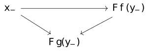
(Note, we use the notation \int for the Grothendieck construction/category of elements, where Buckley uses \mathrm {El})
Constructing the triple category of controlled processes [efr-000G]
- June 14, 2024
-
Eigil Fjeldgren Rischel
Constructing the triple category of controlled processes [efr-000G]
- June 14, 2024
- Eigil Fjeldgren Rischel
Triple categories are very complicated objects. And our life is further complicated by the fact that, in one direction, our triple category is not in general strict, in the sense that composition is only associative up to globular isomorphism (because the tensor product is only pseudoassociative, the composition of controlled processes inherits this defect).
Hence, our life will be greatly simplified if we can approach the construction of this triple category by more conceptual means. Our strategy will essentially be the following:
- We will note that the notion of internal pseudocategory is classified by a limit sketch---that is, there is a bicategory (actually, a 1-category) \mathcal {I} and class of diagrams K so that a pseudocategory internal in \mathcal {C} is precisely a pseudofunctor \mathcal {I} \to \mathcal {C} which carries all the diagrams in K to homotopy limits
- We will prove that the double categorical \mathsf {\mathbb Para}(-) construction preserves homotopy limits.
- Hence, by the preceding point, applying it to a pseudocategory internal to the bicategory of category actions will produce a pseudocategory internal to pseudo double categories---a triple category.
Definition Limit sketch [efr-001M]
- June 25, 2024
-
Eigil Fjeldgren Rischel
Definition Limit sketch [efr-001M]
- June 25, 2024
- Eigil Fjeldgren Rischel
A limit sketch consists of a (small) category \mathcal {I} equipped with a collection of cones (J_i \in \mathsf {Cat}, D_i: J_i^\triangleleft \to \mathcal {I}) (recall that J^\triangleleft is the "cone on J", the result of freely adjoining an initial object to J).
If \mathcal {C} is a category, a model of the limit sketch is a functor M: \mathcal {I} \to \mathcal {C} so that each composite J_i^\triangleleft \to \mathcal {I} \to \mathcal {C} is a limit cone. A morphism of models is any natural transformation. In other words, the category of models is the full subcategory of the functor category spanned by the models. It is denoted \mathsf {Mod}_\mathcal {I}(\mathcal {C}) (the collection of diagrams is left implicit).
Given a bicategory or other higher category \mathcal {C}, a model is a pseudofunctor \mathcal {I} \to \mathcal {C} which carries every diagram to a homotopy limit cone. \mathsf {Mod}_\mathcal {I}(\mathcal {C}) \subseteq \mathsf {Fun}(\mathcal {I},\mathcal {C}) is again the full sub-bicategory of the bicategory of pseudofunctors spanned by the models.
We will see that there are limit sketches classifying both internal categories (giving double categories) and symmetric pseudomonoids (giving symmetric monoidal categories), which will be important going forward.
Remark Pseudocategories and categories of categories [efr-001O]
- June 25, 2024
-
Eigil Fjeldgren Rischel
Remark Pseudocategories and categories of categories [efr-001O]
- June 25, 2024
- Eigil Fjeldgren Rischel
We will want to say that the category of pseudo double categories is the category of internal pseudocategories---modeled as Segal objects---in the bicategory of categories. There are two issues with this statement as written.
First of all, a priori, a weak Segal category is quite different from a pseudo double category. Not only is there not a canonical choice of composition given two horizontal maps f: x \nrightarrow y, g: y \nrightarrow z, we cannot even (a priori) guarantee the existence of a choice of composition gf which has the right boundaries on the nose---only up to vertical isomorphism (so we can find a composite x' \nrightarrow y' and isomorphisms x \cong x', y \cong y'). On the other hand, a weak Segal category is also stronger than a pseudo double category, in the sense that every vertical isomorphism has a companion.
We will see that the first defect can always be remedied after replacing our weak Segal category with an equivalent one. The issue of companions is a fundamental difference, but luckily all of the relevant double categories we want to consider have these companion pairs.
The second question is somewhat subtler (but also less important). The category of internal pseudocategories, computed in any higher category, has a priori the same homotopy level as the input---just as the category of monoids is a 1-category (like \mathsf {Set},) but the category of monoidal categories is a bicategory. This makes sense if we view categories as just a plain (generalized) algebraic theory, but we usually want to think of categories of categories as having some extra homotopy theory coming from the category structure---the category of categories in \mathsf {Set} is a bicategory (actually a 2-category, i.e it's strict), not a plain category. The preceding construction does not account for this---the homotopy limits implicit in the phrase "a pseudocategory in pseudo double categories" are, for us, merely homotopy limits of plain categories, not accounting for the extra categorical structure in a double category.
It is not clear what this means in general (and in any case, our output category will actually be strict in two directions,) but it is an important subtlety to remember.
(A category viewed as an object merely of the 1-category of categories is sometimes called a strict category, but obviously we can't speak about "strict pseudo double categories")
Definition Segal object [efr-001N]
- June 25, 2024
-
Eigil Fjeldgren Rischel
Definition Segal object [efr-001N]
- June 25, 2024
- Eigil Fjeldgren Rischel
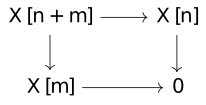
Consider the simplicial category \Delta . For every n,m, the following square commutes:
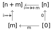
A simplicial object X in a category \mathcal {C} is called a Segal object if each of these squares goes to a pullback square.
Lemma [efr-001P]
- June 25, 2024
-
Eigil Fjeldgren Rischel
Lemma [efr-001P]
- June 25, 2024
- Eigil Fjeldgren Rischel
Let X: \Delta ^\mathrm {op} \to \mathsf {Cat} be a (strict) simplicial category (note that every simplicial category is equivalent to a strict one). Suppose further the face maps X[1] \rightrightarrows X[0] are both isofibrations. Then if X is a Segal category in the strict sense, it is automatically a Segal category in the pseudo sense.
Proof
- June 25, 2024
- Eigil Fjeldgren Rischel
Proof
- June 25, 2024
- Eigil Fjeldgren Rischel
Since, up to isomorphism of categories, the higher X[n] are pullbacks of the two indicated face maps, and the projections in the diagram
Definition Simplicial Category [efr-0016]
- June 24, 2024
-
Eigil Fjeldgren Rischel
Definition Simplicial Category [efr-0016]
- June 24, 2024
- Eigil Fjeldgren Rischel
The simplicial category is the category of finite, nonempty, totally ordered sets, and order-preserving functions, denoted \mathbb {\Delta }. We denote by [n] for n \geq 0 the ordered set \{0 < 1 < \dots < n\} of n+1 elements---every object on \mathbb {\Delta } is isomorphic to one of the form [n].
A simplicial object in a category \mathcal {C} is a functor \Delta ^\mathrm {op} \to \mathcal {C}.
Proposition [efr-0017]
- June 24, 2024
-
Eigil Fjeldgren Rischel
Proposition [efr-0017]
- June 24, 2024
- Eigil Fjeldgren Rischel
Let \mathcal {C} be a category with finite limits. The internal nerve functor \mathsf {Cat}(\mathcal {C}) \to \mathsf {Simp}\mathcal {C} is fully faithful, and the essential image consists exactly of those simplicial objects X where the maps p_i: X[n] \to X[1] given by evaluating at p^i: [1] \to [n] : k \mapsto k+i, i = 0,\dots n-1 exhibits X[n] as the iterated pullback X[1] \times _{X[0]} \dots \times _{X[0]} X[1]
Proposition [efr-0018]
- June 24, 2024
-
Eigil Fjeldgren Rischel
Proposition [efr-0018]
- June 24, 2024
- Eigil Fjeldgren Rischel
A pseudo double category is equivalently a simplicial object in \mathsf {Cat} so that the diagrams X[n] \to X[1] are homotopy pullbacks.
Lemma Commutativity of internalization [efr-001Q]
- June 26, 2024
-
Eigil Fjeldgren Rischel
Lemma Commutativity of internalization [efr-001Q]
- June 26, 2024
- Eigil Fjeldgren Rischel
Let \mathcal {I},\mathcal {J} be limit sketches, and let \mathcal {C} be a bicategory. Then \mathsf {Mod}_\mathcal {I}(\mathsf {Mod}_\mathcal {J}(\mathcal {C})) \simeq \mathsf {Fun}'(\mathcal {I} \times \mathcal {J}, \mathcal {C}) \simeq \mathsf {Mod}_\mathcal {J}(\mathsf {Mod}_\mathcal {I}(\mathcal {C})), where \mathsf {Fun}'(\mathcal {I} \times \mathcal {J},\mathcal {C}) denotes the full subcategory of the functor bicategory spanned by those pseudofunctors F so that, for each I \in \mathcal {I},, F(I,-) is a model of \mathcal {J}, and for each J \in \mathcal {J}, F(-,J) is a model of \mathcal {I}.
Proof
- June 26, 2024
- Eigil Fjeldgren Rischel
Proof
- June 26, 2024
- Eigil Fjeldgren Rischel
Each isomorphism is an immediate consequence of the obvious fact that (pseudo)limits in model (bi)categories are computed pointwise, and the standard currying equivalence.
Remark
- June 26, 2024
- Eigil Fjeldgren Rischel
Remark
- June 26, 2024
- Eigil Fjeldgren Rischel
Remark [efr-001R]
- June 26, 2024
-
Eigil Fjeldgren Rischel
Remark [efr-001R]
- June 26, 2024
- Eigil Fjeldgren Rischel
A weak Segal category is similar to a virtual double category: we don't directly have a composition operator \mathbb {C}_1 \times _{\mathbb {C}_0} \mathbb {C}_1---rather, we have a category of "compositions" \mathbb {C}_2, each of which contains three faces in \mathbb {C}_1. Hence we have a choice of composites for every composable pair, although it is uniquely defined up to contractible choice.
Definition Coherent nerve of pseudo double category [efr-001S]
- June 26, 2024
-
Eigil Fjeldgren Rischel
Definition Coherent nerve of pseudo double category [efr-001S]
- June 26, 2024
- Eigil Fjeldgren Rischel
Let \mathbb {C} be a pseudo double category. Then the coherent nerve is the simplicial category N(\mathbb {C}) defined as follows:
- N(\mathbb {C})_0 = \mathbb {C}_0
- N(\mathbb {C})_1 = \mathbb {C}_1
- The objects of N(\mathbb {C})_2 are tuples f: x \nrightarrow y, g: y \nrightarrow z, h: x \nrightarrow z, \alpha : gf \simeq h, where x,y,z are objects of \mathbb {C}_0, f,g,h are horizontal morphisms, and \alpha is a globular isomorphism in \mathbb {C}_1
- The morphisms of N(\mathbb {C})_2 are triples of 2-cells \phi : f \to f', \psi : g \to g', \xi : h \to h' so that the two possible 2-cells gf \to h' agree
- Given four compatible objects of \N (\mathbb {C})_2 defining a 3-boundary (a tetrahedron), there is a unique objects of \N (\mathbb {C})_3 filling it if and only if the square of globular isomorphisms commute
- Given four compatible morphisms of \N (\mathbb {C})_2, there is always a unique morphism in \N (\mathbb {C})_3 filling the boundary
- The face- and degeneracy functors are the obvious ones
- \N (\mathbb {C}) is 3-coskeletal, which defines the rest of the structure
Theorem [efr-001T]
- June 26, 2024
-
Eigil Fjeldgren Rischel
Theorem [efr-001T]
- June 26, 2024
- Eigil Fjeldgren Rischel
- A pseudo double functor \mathbb {C} \to \mathbb {D} is equivalent to a natural transformation N(\mathbb {C}) \to N(\mathbb {D})
- If \mathbb {C} is a double category in which each vertical isomorphism has a companion, N(\mathbb {C}) is a weak Segal category
- Every weak Segal category is equivalent to one of the form N(\mathbb {C}) for \mathbb {C} a pseudo double category of this type.
Let \mathbb {C} be a double category in which every vertical isomorphism has a companion. Then by
reference here, Shulman stuff,
the source and target functors are isofibrant. To prove N(\mathbb {C}) is a weak Segal category, it therefore suffices to prove that N(\mathbb {C})[2] \to N(\mathbb {C})[1] \times _{N(\mathbb {C})[0]} N(\mathbb {C})[1] is an equivalence of categories, and the analogous statement in level 3 (it follows for the higher levels by coskeletality).Now, let X be a weak Segal. By
reference
, every simplicial category is equivalent to one which is Reedy fibrant. Note that being a Segal category is preserved by equivalence, so without loss of generality, assume X is Reedy fibrant.This means the functor X[n] \to X(\partial \Delta ^n) is an isofibration for each n. First, let n=1. This means X[1] \to X[0] \times X[0] is an isofibration. Since such fibrations are stable under pullback, this implies that the projection X(\partial \Delta ^2) \to X[1] \times _{X[0]} X[1] is again an isofibration, which means the composite X[2] \to X[1] \times _{X[0]} X[1] is an isofibration. Since this pullback is a homotopy pullback, and X is weak Segal, it is an equivalence, and hence a trivial equivalence. Choose a (strict!) section s.
By a completely analogous argument, choose a section of X[3] \to X[1] \times _{X[0]} X[1] \times _{X[0]} X[1], which is again a trivial fibration.
Let our pseudo double category have X[1] \rightrightarrows X[0] as the underlying reflective graph, composition defined by the composite X[1] \times _{X[0]} X[1] \to X[2] \xrightarrow {d_1} X[1], associator defined using the degeneracies, and unitor defined using the section of X[3]. Call this pseudo double category \mathbb {X}
It is easy to see there is a functor X \to N(\mathbb {X}), which is the identity on the first two levels. Since the higher levels are homotopy pullbacks of the lower levels, this implies it is an equivalence at each level, concluding the proof.
Theorem \dblPara preserves homotopy limits [efr-000H]
- June 14, 2024
-
Eigil Fjeldgren Rischel
Theorem \dblPara preserves homotopy limits [efr-000H]
- June 14, 2024
- Eigil Fjeldgren Rischel
The pseudofunctor \mathsf {\mathbb Para}: \mathsf {Arr}(\mathsf {SymMonCat}) \to \mathsf {PsDbl}, which carries a symmetric monoidal functor \mathcal {C} \to \mathcal {D} to the pseudo double category \mathsf {\mathbb Para}_\mathcal {C}(\mathcal {D}), preserves homotopy limits.
Proof
- June 14, 2024
- Eigil Fjeldgren Rischel
Proof
- June 14, 2024
- Eigil Fjeldgren Rischel
Note that homotopy limits on both sides are computed levelwise (using the observation that both are categories of models of (homotopy) limit sketches in the bicategory \mathsf {Cat}.)
Since \mathsf {\mathbb Para}_\mathcal {C}(\mathcal {D})_0 = \mathcal {D}, this immediately implies that \mathsf {\mathbb Para}(-)_0 preserves homotopy limits. It suffices to verify that \mathsf {\mathbb Para}(-)_1 also preserves them. But note that \mathsf {\mathbb Para}_\mathcal {C}(\mathcal {D})_1 can be written as the comma object of the cospan \mathcal {C} \times \mathcal {D} \to \mathcal {D} = \mathcal {D}, and since comma objects are PIE limits, they commute with homotopy limits (pseudolimits). This concludes the proof.
Note that (pseudo-) monoids M equipped with a left module C in a general bicategory \mathcal {C} are also classified by a limit sketch, and both the underlying object of the module and the map C \times M \to M are in the image of this limit sketch. By instantiating this for \mathcal {C} being the bicategories of categories (or monoidal categories, etc), we recover alternative versions of Theorem [efr-000H] for category actions that are not symmetric. We will mainly concern ourselves with the symmetric case, however.
Definition \mathsf {\mathbb Ctrl} [efr-000I]
- June 14, 2024
-
Eigil Fjeldgren Rischel
Definition \mathsf {\mathbb Ctrl} [efr-000I]
- June 14, 2024
- Eigil Fjeldgren Rischel
Let \mathcal {C}, \mathcal {A}(-), T be a dynamical systems theory, let \mathsf {\mathbb Arena} be the associated category of arenas. Recall that \mathsf {\mathbb Arena}_0 is the category of lenses.
Consider the (strict) category internal to \mathsf {Arr}(\mathsf {SymMonCat}) given by the following diagram:
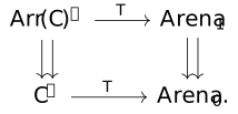
(Note the difference between \mathsf {Arr}(\mathcal {C})^\simeq and \mathsf {Arr}(\mathcal {C}^\simeq )---the former has objects all morphisms of \mathcal {C}, and the morphisms between them given by isomorphisms, whereas the latter has objects only the isomorphisms in \mathcal {C})
Proposition [efr-000J]
- June 14, 2024
-
Eigil Fjeldgren Rischel
Proposition [efr-000J]
- June 14, 2024
- Eigil Fjeldgren Rischel
The objects of \mathsf {\mathbb Ctrl} are arenas.
The three directions of morphism in \mathsf {\mathbb Ctrl} are lenses, charts, and controlled processes.
The lens-chart double category is isomorphically \mathsf {\mathbb Arena}---in particular, composition of both lenses and charts is strictly associative.
The process-chart double category has 2-cells the chart reparametrizations. The process-lens double category has 2-cells the lens isoparametrizations. They both compose in the obvious way.
Processes compose as morphisms of \mathsf {Para}_{\mathcal {C}^\simeq }(\mathsf {Lens})---that is, (S,TS \otimes A \to B) ; (S', TS' \otimes B \to C) = (S' \otimes S, T(S' \otimes S) \otimes A \cong TS' \otimes TS \otimes A \to TS' \otimes B \to C), this is associative up to a coherent choice of globular isoparametrization.
[efr-000U]
- June 17, 2024
-
Eigil Fjeldgren Rischel
[efr-000U]
- June 17, 2024
- Eigil Fjeldgren Rischel
We can consider two strategies for constructing the "full" triple category of controlled processes:
- Give a construction of the double category of controlled processes and all lens reparametrizations, in a functorial way so that we can extend this to a triple category
- Prove that freely(?) adding companions, in a suitable sense, of each globular chart reparametrization, gives the right thing (this should amount to checking a composition rule)
Proposition [efr-000V]
- June 17, 2024
-
Eigil Fjeldgren Rischel
Proposition [efr-000V]
- June 17, 2024
- Eigil Fjeldgren Rischel
Let \mathsf {\mathbb Ctrl}_1 \to \tilde {\mathsf {\mathbb Ctrl}_1} be constructed by freely adding companions of every globular chart reparametrization. Then \tilde {\mathsf {\mathbb Ctrl}_1} admits the following description:
- The objects are the objects of \mathsf {\mathbb Ctrl}_1, i.e tuples A,B,S, TS \otimes A \leftrightarrows B
- The vertical morphisms are chart reparametrizations
- The horizontal morphisms are lens reparametrizations
- \mathsf {\mathbb Ctrl}_1 is thin, and a square exists if and only if the underlying square in \mathcal {C} commutes.
Fix the notation of \mathsf {\mathbb Ctrl} vs \tilde {\mathsf {\mathbb Ctrl}}
Proof
- June 17, 2024
- Eigil Fjeldgren Rischel
Proof
- June 17, 2024
- Eigil Fjeldgren Rischel
insert example here
, we have seen that every lens reparametrization factors as a composite of companions of lens isoparametrizations and companions of globular chart reparametrizations...finish this
.
proposition [efr-000X]
- June 20, 2024
-
Eigil Fjeldgren Rischel
proposition [efr-000X]
- June 20, 2024
- Eigil Fjeldgren Rischel
The functor A \otimes -: \mathsf {BorelStoch} \to \mathsf {BorelStoch} has a terminal coalgebra, carried by A^\omega with the deterministic structure map \langle \rm head, tail \rangle : A^\omega \to A \otimes A^\omega .
Proof
- June 20, 2024
- Eigil Fjeldgren Rischel
Proof
- June 20, 2024
- Eigil Fjeldgren Rischel
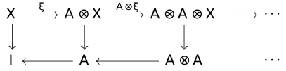
Observe that this diagram is a Kolmogorov limit in \mathsf {BorelStoch}:

This gives a coalgebra structure on A^\omega in the usual way.
Given \xi : X \to X \otimes A, we can build a cone by iteratively applying A \times - to the unique map X \to I:
The Double Category of Stochastic Arenas [efr-001L]
- June 25, 2024
-
Eigil Fjeldgren Rischel
The Double Category of Stochastic Arenas [efr-001L]
- June 25, 2024
- Eigil Fjeldgren Rischel
Let \mathcal {D} \to \mathcal {C}_\mathrm {det} be a Markov fibration. Since it is a fibration, we may form the ordinary double category of arenas \mathsf {\mathbb Arena}(\mathcal {D}). Note that there is a double functor \mathsf {\mathbb Arena}(\mathcal {D}) \to \mathcal {C}_\mathrm {det}^\square . This is a double fibration: an internal category in the category of fibrations.
The double category of stochastic arenas is obtained by stochastically completing this fibration in both directions---in other words, we form the completions \overline {\mathsf {\mathbb Arena}(\mathcal {D})_1} and \overline {\mathsf {\mathbb Arena}(\mathcal {D})_2}. We must check that this still gives a double category (it does), which we then transpose, stochastically complete, then transpose again (once again, there is something to check to see that the completion preserves the double categorical structure).
The phrase "stochastic arenas" is a bit unfortunate, since the arenas themselves are no different from ordinary arenas (stochastic completion does not change the objects). Rather, it is the morphisms, the lenses and charts, that are stochastic.
Definition Stochastic lens [efr-002S]
- July 4, 2024
-
Eigil Fjeldgren Rischel
Definition Stochastic lens [efr-002S]
- July 4, 2024
- Eigil Fjeldgren Rischel
Let \mathcal {D} \to \mathcal {C} be a stochastically complete Markov fibration. Then a stochastic lens \bar {X} \to \bar {Y}, where \bar {X},\bar {Y} \in \mathcal {D}, with p(\bar {X}) = X, p(\bar {Y}) = Y, consists of:
- An object M \in \mathcal {C}, equipped with deterministic maps p_X: M \to X, p_Y: M \to Y
- A (non-deterministic) section s: X \to M of p_X
- And a map \phi : p_Y^*\bar {Y} \to \bar {X} over p_X
- Up to the equivalence relation identifying two such tuples (M,p_X,p_Y,s,\phi ), (N,q_X,q_Y,t,\psi ) if there exists (non-deterministic) \alpha : M \to N so that the relevant diagrams commute---that is, the projections to X and Y commute with \alpha , t= \alpha s, and \phi = \psi \bar {\alpha }, where \bar {\alpha }: p_Y^*\bar {Y} \to q_Y*\bar {Y} is the unique map induced by the stochastic completeness property
(This could have been described as a coend, but since we don't find the coend calculus very useful for manipulating the set of stochastic lenses, we choose not to.)
Given an optic, the forwards part is the composite map X \to M \to Y.
The opposite of \mathsf {FinStoch} [efr-0030]
- July 15, 2024
-
Eigil Fjeldgren Rischel
The opposite of \mathsf {FinStoch} [efr-0030]
- July 15, 2024
- Eigil Fjeldgren Rischel
Recall that (perhaps by definition, perhaps as a trivial theorem, depending on our choice of definition), there is a faithful functor \mathsf {FinStoch} \to \mathsf {Vect} carrying a set X to the vector space \mathbb {R}\langle X \rangle freely generated by X, and a stochastic map f: X \to Y to the map which takes the basis vector x \in X to the linear combination \sum _{y \in Y} y f(y|x). The essential image of this functor is, of course, the finite-dimensional vector spaces. The morphisms in the image are the stochastic matrices, which can be characterized as those that are positive (they carry vectors with positive coordinates to other such vectors) and preserve the constant 1 vector (note that neither of these properties are invariant under isomorphism of finite-dimensional vector space).
One way to think about this is that it proves \mathsf {FinStoch} is equivalent to the category of finite-dimensional, ordered, pointed vector spaces, where we assume that the chosen point must be positive in the order. (To see the inclusion is essentially surjective, note that given a vector space pointed by (a_1, \dots a_n), all those coordinates positive, it receives an isomorphism from the same spaces pointed by (1, \dots 1) given by the diagonal matrix with entries a_1, \dots a_n).
Now, let \mathsf {fdVect}^\leq denote the category of finite-dimensional ordered vector spaces. Then equipping a space V with a positive point is exactly choosing an order-preserving linear map \mathbb {R} \to V, so we have proven \mathsf {FinStoch} \simeq \mathsf {fdVect}^\leq _{ \mathbb {R} /}. Now we can compute \mathsf {FinStoch}^\mathrm {op} \simeq (\mathsf {fdVect}^\leq _{ \ RR/})^\mathrm {op} \cong (\mathsf {fdVect}^\leq )^\mathrm {op}_{ / \mathbb {R}} \cong \mathsf {fdVect}^\leq _{ / \mathbb {R}}, where the last isomorphism is via transposition (note that transposing a positive matrix yields a positive matrix).
This isomorphism merely describes the fact that stochastic maps \phi : X \to Y can also be described as linear maps f: \mathbb {R}\langle Y \rangle \to \mathbb {R}\langle X \rangle so that \sum _x f((a_y))_x = \sum _y a_y. This map interprets a vector as a function on Y, and carries it to the function on X which finds the expected value if y \in Y is distributed as \phi (x). The normalization condition merely says a constant function always has that constant as its expectation.
The self-duality of \mathsf {fdVect} does not generalize to infinite-dimensional vector spaces, so once we move beyond finite state spaces, this story will get somewhat more complicated. However, the basic idea that, to carry the tools of coalgebraic modal logic into the stochastic case, the sort of "predicate" we should consider is actually a function on the state space, will remain the central idea.
(Indeed, to consider the right notion of stochastic function between, for example, smooth manifolds, we will in any case want to use the tools of functional analysis to think of these in terms of transformation on integration operators, which is essentially this idea).
Another way to justify this idea is to note that \Omega = \{\bot ,\top \} is the subobject classifier for \mathsf {Fin} \subseteq \mathsf {FinStoch}. Hence if we want our notion of predicate to transform under stochastic maps, and include the logical predicates in the usual sense, we have to at least consider the stochastic maps X \to \Omega , which of course amount to functions X \to [0,1] in this case. But a positive linear map on functions is determined by what it does to functions like this, so whether we work only with these or all functions X \to \mathbb {R} is more or less a matter of taste.
Instead of having a logic consisting of the operations of Boolean algebra, augmented with extra operations described by T^\mathrm {op} B \to B, we have the operations of a vector space, augmented by some extra modal operations. The Markov structure of \mathsf {FinStoch}, or whichever category we work in, will give the vector space of functions an \mathbb {R}-algebra structure, but we should note that some equations fail to hold in general (dual to the fact that not all morphisms in the Markov category are homomorphisms for the comonoid structure). The Hennessy-Milner property is essentially the same in this situation, saying that our set of modally-expressible functions should separate points in the terminal coalgebra. Since we will have multiplication and linear combinations of functions, this entails under some mild topological conditions that it's dense in the set of functions on the terminal coalgebra.
It is worth examining this analogy a bit further, in the simpler setup of coalgebraic modal logic. If X is a space in some general sense, let us schematically write C(X) for the space of functions on X, so that as above stochastic maps X \to Y are identified with certain linear maps C(Y) \to C(X). Again, the Markov structure on the category of stochastic maps (whatever it is) amounts to the fact that C(X) carries the structure of an \mathbb {R}-algebra, and deterministic maps are those which are not algebra homomorphisms.
Let now \xi : X \to A \otimes X be a simple stochastic dynamical system which outputs a value of type A at each step. The dual of this is C(A) \otimes C(X) \to C(X), where the tensor here is now the tensor product of vector spaces.
Among algebras, the tensor product is the coproduct, so we may restrict the above map to form two modal operators, C(A) \to C(X) and C(X) \to C(X)---the latter being simply the transition operator taking a function \phi (x) to the expected value of the next step, the former computing the expected value of the output given x. But since the transition may be nondeterministic, these two restrictions do not determine it. From a logical point of view, the problem is that we can't express statements about the correlation between the output and the next step.
As a simple counterexample, consider two system where X = A = \{0,1\}. In the first, the output and the next state are independent, and both equal the current state with probability 1-\epsilon . In the other, the output and next state are always equal, and again are equal to the current state with probability 1-\epsilon
These systems have the same marginals X \to A and X \to X, and hence the two modal operators above have the same behaviour, and hence every modally expressible function is the same. But in the former, the probability of seeing ab output sequence beginning 1,0,\dots when starting in state 0 is proportional to \epsilon , whereas in the latter it is proportional to \epsilon ^2 (since you have to flip twice), so these systems have very different behaviour.
Using § [efr-000X], we can deduce a version of Hennessy-Milner for stochastic transition systems (with no input and outputs in finite set A). Namely, fix a system \xi : X \to A \otimes X, and let \nabla (u,v), with u: A \to \mathbb {R} and v: X \to \mathbb {R} denote the function which carries x \in X to the expected value of u(a)v(x') when (a,x') are distributed according to the system. Then \nabla is precisely the bilinear function C(A) \otimes C(X) \to C(X) dual to \xi . Since A^\omega is the terminal coalgebra, and the inverse limit of A \leftarrow A^2 \leftarrow \dots , we can infer that C(A^\omega ) is the colimit of the sequence C(A) \to C(A) \otimes C(A) \to \dots in some category of \mathbb {R}-algebras (we must think a little about topology to make this precise.)
But this should imply that the union of the images of C(A)^{\otimes n} inside this algebra is dense. So certainly they separate points. But this image consists exactly of formulas given by functions on A, applications of \nabla , and sums and products. So these formulae are sufficiently expressive to separate points of the terminal coalgebra (which are, of course, exactly bisimulation classes).
Logic for systems misc
- November 19, 2024
-
Eigil Fjeldgren Rischel
Logic for systems misc
- November 19, 2024
- Eigil Fjeldgren Rischel
Stochastic Categorical Systems Theory (The Discrete Case) [efr-001B]
- June 24, 2024
-
Eigil Fjeldgren Rischel
Stochastic Categorical Systems Theory (The Discrete Case) [efr-001B]
- June 24, 2024
- Eigil Fjeldgren Rischel
It will be instructive to work out the theory in the discrete case, which is to say, for the Kleisli category of the discrete (i.e finite-support) distribution monad on \mathsf {Set}. Note that even for discrete-time discrete-space applications, this setup is not really adequate, as we lack the structure to construct terminal systems.
Definition [efr-001C]
- June 24, 2024
-
Eigil Fjeldgren Rischel
Definition [efr-001C]
- June 24, 2024
- Eigil Fjeldgren Rischel
Let \Delta : \mathsf {Set} \to \mathsf {Set} carry a set X to the set of finite-support probability distributions on X. Recall that \Delta is a monad.
Given two indexed sets \bar {X} \to X, \bar {Y} \to Y, an indexed stochastic lens \binom {\bar {X}}{X} \to \binom {\bar {Y}}{Y} is an element of the convex space \prod _{x \in X} \sum _{y \in Y} [\Delta (\bar {Y}_y),\Delta (\bar {X}_x)], where the internal hom, product and coproduct are taken in the category of convex spaces. Note that if each \bar {Y}_y is identical, say B, this is isomorphism to \prod _{x \in X} \Delta (Y) \otimes [\Delta (B),\Delta (\bar {X}_x)]. Recall also that an element of [\Delta (X),\Delta (Y)] is equivalently a function X \to \Delta (Y), i.e. a Kleisli map X \to Y.
An indexed stochastic chart is an element of the convex space \prod _{x \in X} \sum _{y \in Y} [\Delta (\bar {X}_x),\Delta (\bar {Y}_y)]
Proposition [efr-001D]
- June 24, 2024
-
Eigil Fjeldgren Rischel
Proposition [efr-001D]
- June 24, 2024
- Eigil Fjeldgren Rischel
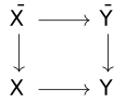
The set of indexed stochastic charts is just the set of commutative squares in \mathsf {Kl}(\Delta ) of this form:
Proof
- June 24, 2024
- Eigil Fjeldgren Rischel
Proof
- June 24, 2024
- Eigil Fjeldgren Rischel
where this exponential denotes the iterated Cartesian product in convex spaces. An element of this set clearly gives a commutative square, because for each y \in Y, there is a square which deterministically chooses that y, and uses the given family of distributions on \bar {Y}_y depending on \bar {X}. This mapping is injective, since each map \bar {X} \to \Delta (\bar {Y}_y) can be recovered as a conditional distribution, and the convex combination of ys is merely the underlying distribution on Y. On the other hand, by choosing conditional distributions, it is also seen to be surjective, finishing the proof.
Quantitative logic for systems [efr-001W]
- June 28, 2024
-
Eigil Fjeldgren Rischel
Quantitative logic for systems [efr-001W]
- June 28, 2024
- Eigil Fjeldgren Rischel
Definition [efr-001V]
- June 28, 2024
-
Eigil Fjeldgren Rischel
Definition [efr-001V]
- June 28, 2024
- Eigil Fjeldgren Rischel
Let \alpha : TS \leftrightarrows A be a system with interface A, and let P be another arena.
A P-valued predicate on \alpha is a lift
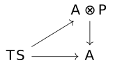
For discrete-time deterministic systems, a P = {\bar {P} \choose P}-valued predicate amounts to a mapping S \to P---since the diagram implies the update can't depend on the extra input \bar {P}, and in the deterministic case, a lift of S \to A over A \otimes P is simply a choice of S \to P. (In the non-deterministic case, this is not true, of course).
Let F: \mathsf {Set} \to \mathsf {Set} be a functor, and let \xi : X \to FX be a coalgebra of it. Then we can describe a predicate of X valued in P \in \mathsf {Set} as simply a function \phi : X \to P. Note that this makes X a coalgebra of F(-) \times P, and as such it has a unique map to the terminal coalgebra (if it exists) of this functor X \to (F(-) \times P)^\infty .
This means, given a predicate on that terminal coalgebra, p: (F(-) \times P)^\infty \to P, by composing these two operations, we get a new predicate on X. Thus, predicates on these cofree coalgebras are a sort of "modal operators"---for example, if P = \{\bot ,\top \} is the set of booleans, and F(X) = X (so that coalgebras are just discrete dynamical systems), the cofree coalgebra on P is the set \{\bot ,\top \}^\omega of streams of booleans. Then we can take p((\phi _i)) to be true if and only if each \phi _i is true. Then the modal operator of p is essentially "necessity"---the composite predicate is true for exactly those x \in X so that \phi (x_n) is true for every x_n on the trajectory.
Definition [efr-001X]
- June 28, 2024
-
Eigil Fjeldgren Rischel
Definition [efr-001X]
- June 28, 2024
- Eigil Fjeldgren Rischel
Let p: A' \leftrightarrows A be a lens, let T(A')^\infty \leftrightarrows A' be the terminal A'-system, and consider the composite T(A')^\infty \leftrightarrows A' \leftrightarrows A. A A'/A-modal operator is a factorization of this system over A' \leftrightarrows A, i.e some other A'-system with the same state space, \alpha : T(A')^\infty \leftrightarrows A' so that the two composites T(A')^\infty \leftrightarrows A' \leftrightarrows A agree.
Let \xi : TS \to A' be some other system. It has a unique map to the terminal system. After composing with p: A' \leftrightarrows A, we can regard this as a map p\xi \to p\alpha . We can then compose this with the unique map from \alpha to the terminal system, obtaining a new map p(\xi ) \to p((A')^\infty ). This is the operation corresponding to \alpha .
In good cases, there will be a monadic adjunction associated to the lens A' \leftrightarrows A, and so this operation will give an endomorphism on predicates for each choice of lift of the cofree predicate (it can of course lift as itself, which corresponds to the identity operation).
[efr-001Y]
- June 28, 2024
-
Eigil Fjeldgren Rischel
[efr-001Y]
- June 28, 2024
- Eigil Fjeldgren Rischel
When moving from deterministic, ordinary differential equations, to stochastic differential equations---or, from another point of approach, moving from discrete-time stochastic systems to continuous-time stochastic systems---we are forced to confront the problem that typical stochastic differential equations do not have differentiable solutions.
A few questions immediately pose themselves when confronted with this statement:
- Since a solution of a stochastic differential equation is not merely a function but some sort of distribution of functions, what do you mean by them not being differentiable?
- Whatever the solutions are, how can they solve a differential equation if they aren't't differentiable?
It will be instructive to consider Brownian motion. For each t \in \mathbb {R}, let E_t be an independent standard Gaussian. There are some issues with defining the integral X_r = \int _0^r E_t dt, since t \mapsto E_t can't be guaranteed to be even measurable, but these can be sidestepped without too many problems. Then X_r is Brownian motion, but with probability 1 it is nowhere differentiable. The integral equation above describes the sense in which X solves a stochastic differential equation saying it's derivative at each point is standard Gaussian distributed.
Of course, since not all systems are integrable (this is not even true in the deterministic case,) there is not gonna be an integral operator lying around that we can use to define the solutions of our differential equations. Hence we must use a different solution concept.
Recall that, if f,g: \mathbb {R} \to \mathbb {R} are differentiable functions, \int _a^b f(x)g'(x)dx = f(a)g(a)---f(b)g(b)---\int _a^b f'(x)g(x)dx, (integration by parts). Now if we choose f to be zero except on a bounded interval, and let the endpoints to infinity, we get \int _\mathbb {R} f(x)g'(x) dx =---\int _\mathbb {R} f'(x)g(x)dx. The trick here is that the right-hand side is defined even if g is not differentiable, and so it gives us a way of talking about "the derivative of g", at least for some purposes, even when it doesn't exist.
Since two functions have the same integral after multiplication by every differentiable f, if and only if they're equal almost everywhere, this is fairly robust---if g is C^1 and satisfies some differential equation "weakly", it follows it must satisfy it on the nose as well, for example.
Theorem Riesz Representation [efr-001Z]
- June 28, 2024
-
Eigil Fjeldgren Rischel
Theorem Riesz Representation [efr-001Z]
- June 28, 2024
- Eigil Fjeldgren Rischel
Let X be a locally compact Hausdorff topological space, and let C_c(X) denote the vector space of complex-valued, compactly supported functions on X. Recall that a linear functional \psi : C_c \to \mathbb {C} is positive if it carries functions valued in the nonnegative reals to nonnegative real numbers.
For every positive linear functional \psi , there exists a unique Radon measure \mu on X so that \psi (f) = \int _X f(x)d\mu (x) (conversely, it is clear that given a Radon measure, this equation defines a positive linear functional).
Let \phi : C_c(Y) \to C_c(X) be a positive linear map. Then dualizing gives a linear map \phi ^*: C_c(X)^* \to C_c(Y)^*. If we assume the initial map preserves the constant 1 function, this will preserve probability measures, making it a sort of infinity-dimensional stochastic matrix.
In particular, we get a composite map X \to C_c(X)^* \to C_c(Y)^*, where the first map just includes the dirac measures (or, alternatively, takes x to the "evaluate at x" functional).
If we further assume \phi is continuous for the uniform convergence topology, \phi ^* will be continuous for the pointwise convergence topology. Since every probability measure is a limit of linear combinations of dirac measures in this topology, that means \phi ^* will be controlled by the above map, so we really have an injective correspondence between linear, continuous and unit-preserving maps C_c(Y) \to C_c(X) and some subset of the Markov kernels X \to Y.
If we stare at this sequence of composites a bit, we realize that the linear operation corresponding to a kernel pX \to Y carries a function f: Y \to \mathbb {R} to the expected value function x \mapsto E_{y \sim p(x)} f(y). Not all Markov kernels will have the property that this preserves continuity of f (all measurable functions are Markov kernels, even)---but we would probably want to impose some notion of continuity on our kernels in any case.
Instead of thinking about the classes of Markov kernels with this continuity-of-expectation property, we can simply use the space of continuous, unit-preserving linear maps C_c(Y) \to C_c(X) as our class of stochastic maps X \to Y.
SDEs are only diffusion and drift [efr-0020]
- June 29, 2024
-
Eigil Fjeldgren Rischel
SDEs are only diffusion and drift [efr-0020]
- June 29, 2024
- Eigil Fjeldgren Rischel
Naively, we would think that a stochastic differential equation on a manifold X should be a stochastic section of the tangent bundle, f: X \to \Delta (TX) (with the understanding that such a thing may not always have a solution).
Indeed, we will see that such a thing does lead to a differential equation. But unlike the deterministic case, there is not a 1-1 correspondence---different sections may determine the same differential equation (in the sense of having the same solutions).
The issue is that, as we have discussed, by necessity solutions of stochastic differential equations are defined by integration, in a certain sense. The solution concept we have in mind is a Markov process, where each derivative is sampled independently from its distribution. But by the central limit theorem, integrating a family of independent random variables will always give a normal distribution, no matter what those variables are.
In particular, the only aspect of the assigned distribution of derivatives f(x) \in \Delta (T_xX) is its mean Ef(x) \in T_xX and its covariance matrix, which is the expectation of v \otimes v inside the tensor product T_xX \otimes T_xX when v \sim f(x).
(Another way of viewing the covariance is as an operator on the tensor product of the covector space T_x^*X \otimes T_x^*X \to \mathbb {R}, which carries a simple tensor of two covectors \phi \otimes \psi to the expected value of \phi (v)\psi (v) when v is sampled according to the given distribution).
[efr-0021]
- June 29, 2024
-
Eigil Fjeldgren Rischel
[efr-0021]
- June 29, 2024
- Eigil Fjeldgren Rischel
In our study of discrete-time systems, we used the observation that the terminal system with a given interface can be characterized as the set of trajectories of that interface (eg § [efr-000X]). This allows us to develop an algebra of predicates on systems in the vein of coalgebraic modal logic.
However, for continuous-time systems, the situation is much more complicated. In general, we can't expect an ordinary differential equation to have a unique solution for each initial value. There are two basic reasons for this:
- A simple system like y' = y^2, y \in \mathbb {R} experiences finite-time blowup, escaping to infinity inside a finite time horizon. In this example, the solutions have the form y(t) = 1/(t+C), and so they clearly can't be continued past a certain horizon. Given some function \alpha (y), we can't extend this to a function t \mapsto \alpha (y(t)) on all of \mathbb {R}
- The differential equation y' = 2 \sqrt {|y|} has both the solution y(t) = 0 and y(t) = y^2 (and many others)
The second issue can be solved by assuming our equations are Lipschitz (which the square root function is not). Since smooth functions are at least Lipschitz on compact domains (with Lipschitz constant bounded by the maximal derivative), there is some hope that we can get rid of this problem (but note that, when studying stochastic processes, there are reasons for wanting to study processes with jumps, complicating the situation).
However, the first issue is more resilient. One approach is to restrict our attention to compact manifolds---this is enough to guarantee that every smooth differential equation has a (global) solution. The problem with this is that the spaces of trajectories---like the space of smooth functions \mathbb {R} \to A---will not even be a manifold, but some type of generalized smooth space. Hence we will not a priori be able to extend this class
Theorem [efr-0022]
- June 29, 2024
-
Eigil Fjeldgren Rischel
Theorem [efr-0022]
- June 29, 2024
- Eigil Fjeldgren Rischel
Consider the category of smooth microlinear spaces X equipped with a map X \to A and a vector field X \to TX.
- This category has a terminal object, given by the colimit taken over a suitable class of small objects. In other words, a point in the terminal system is given by some system U \to TU \times A and a point u_0 \in U, up to an equivalence relation of bisimulation
- The mapping space A^R, equipped with the evaluation at 0 map A^R \to A and the flow \frac {du}{dt} = \frac {du}{dx} is a subterminal object.
- A system X \to A \times TX admits a map to A^R if and only if it is integrable in both directions
Review of coalgebraic modal logic [efr-002A]
- July 1, 2024
-
Eigil Fjeldgren Rischel
Review of coalgebraic modal logic [efr-002A]
- July 1, 2024
- Eigil Fjeldgren Rischel
Definition Weak limits [efr-002B]
- July 1, 2024
-
Eigil Fjeldgren Rischel
Definition Weak limits [efr-002B]
- July 1, 2024
- Eigil Fjeldgren Rischel
Let X: I \to \mathcal {C} be a diagram. A cone A \xrightarrow {f_i} X_i is said to be a weak limit if, for any other cone B, there exists a map B \to A (but this map is not necessarily unique).
Observe that, if an actual limit L exists, a cone is a weak limit if and only if the induced map A \to L admits a section. It follows that any functor which preserves the limit of some diagram also preserves the weak limits (in the sense that they are carried to another weak limit).
Proposition [efr-002C]
- July 1, 2024
-
Eigil Fjeldgren Rischel
Proposition [efr-002C]
- July 1, 2024
- Eigil Fjeldgren Rischel
Let T: \mathsf {Set} \to \mathsf {Set} be a functor which preserves weak pullbacks. Then the assignment \bar {T}(R: A \nrightarrow B) = im(T(R)) \subseteq T(A) \times T(B) defines a functor \mathsf {\mathbb Rel} \to \mathsf {\mathbb Rel} (which just acts as T on the objects).
Proof
- July 1, 2024
- Eigil Fjeldgren Rischel
Proof
- July 1, 2024
- Eigil Fjeldgren Rischel
Recall that there is a functor \mathsf {\mathbb Span}(\mathsf {Set}) \to \mathsf {\mathbb Rel}, which carries a span A \leftarrow R \to B to its image inside A \times B. Observe that two spans are identified under this mapping precisely if there exist span maps (not necessarily inverses) between them in both directions.
It follows that, given two composable relations R: A \nrightarrow B, R': B \nrightarrow C, the composite of \bar {T}(R) and \bar {T}(R') can be computed by taking the pullback T(R) \times _{T(B)} T(R'), then taking its image inside T(A) \times T(C). But since T preserves weak limits, the map from T(R \times _B R') to this pullback admits a section, and hence they go to the same relation. This proves that \bar {T} preserves composition (the claim about identities is straightforward).
The basic idea is the following: suppose we have a system of formula L we know how to interpret in coalgebras. This interpretation is a relation \vDash : L \nrightarrow X, given some coalgebra \xi : X \to TX. Now, given an element \alpha \in TL, we can define its interpretation in TX simply using the lifting \bar {T}. And finally we can take the inverse image of the given subset of TX under \xi to give a subset of X
For example, let T(X) = A \times X, so that a coalgebra is a simple labeled transition system. Then we get a modal operator \nabla _a for each a. The meaning of \nabla _a(\phi )(x) is that \xi (x) = (a,x'), and \phi (x') holds.
If we let our basic language be Boolean logic, and our functor T is not too bad (for example, if it's finitary), we get a result called the Hennessy-Milner property: two states satisfy the same formulae of the logic precisely if they are bisimilar.
(It is not quite the same as saying formulas up to semantic equivalence are the same as bisimilarity classes---in the above example, we only get to ask about some finite prefix of the stream of outputs produced by x. But of course two streams are equal if all the prefixes agree).
Let \mathsf {Stone} denote the category of stone spaces, that is topological spaces which are compact, Hausdorff, and totally disconnected (meaning every connected component is a singleton). Then we have the following theorem, due to Stone
Theorem Stone duality [efr-002D]
- July 1, 2024
-
Eigil Fjeldgren Rischel
Theorem Stone duality [efr-002D]
- July 1, 2024
- Eigil Fjeldgren Rischel
If X is a Stone space, the set of clopen subsets is a Boolean algebra. Moreover, the functor \mathsf {Stone}^\mathrm {op} \to \mathsf {Bool} which carries a Stone space to its set of clopen subsets is an equivalence of categories.
Now suppose our behaviour is given by an endofunctor T: \mathsf {Stone} \to \mathsf {Stone}. Then we immediately get a corresponding functor T^\mathrm {op}: \mathsf {Bool} \to \mathsf {Bool}, and the category of T-coalgebras is dual to the category ot T^\mathrm {op}-algebras.
Hence, giving a space the structure of a T-coalgebra \xi : X \to TX is equivalent to giving its set of clopen subsets a T^\mathrm {op}-algebra structure T^\mathrm {op} B(X) \to B(X). This algebra structure can be interpreted as a (system of) modal operators---for example, if T(X) = A \times X, giving such a structure amounts to choosing maps B(A) \to B(X) and B(X) \to B(X), corresponding to the operations "will x produce an output a that satisfies statement \phi (a)?" and "will the next state after x satisfy \psi ?"
We would like to move this framework to the setting of categorical systems theory. Of course, we are hampered by two immediate problems: our systems are not, in general, coalgebras of functors, nor are they in general sets.
The opposite of \mathsf {FinStoch} [efr-0030]
- July 15, 2024
-
Eigil Fjeldgren Rischel
The opposite of \mathsf {FinStoch} [efr-0030]
- July 15, 2024
- Eigil Fjeldgren Rischel
Recall that (perhaps by definition, perhaps as a trivial theorem, depending on our choice of definition), there is a faithful functor \mathsf {FinStoch} \to \mathsf {Vect} carrying a set X to the vector space \mathbb {R}\langle X \rangle freely generated by X, and a stochastic map f: X \to Y to the map which takes the basis vector x \in X to the linear combination \sum _{y \in Y} y f(y|x). The essential image of this functor is, of course, the finite-dimensional vector spaces. The morphisms in the image are the stochastic matrices, which can be characterized as those that are positive (they carry vectors with positive coordinates to other such vectors) and preserve the constant 1 vector (note that neither of these properties are invariant under isomorphism of finite-dimensional vector space).
One way to think about this is that it proves \mathsf {FinStoch} is equivalent to the category of finite-dimensional, ordered, pointed vector spaces, where we assume that the chosen point must be positive in the order. (To see the inclusion is essentially surjective, note that given a vector space pointed by (a_1, \dots a_n), all those coordinates positive, it receives an isomorphism from the same spaces pointed by (1, \dots 1) given by the diagonal matrix with entries a_1, \dots a_n).
Now, let \mathsf {fdVect}^\leq denote the category of finite-dimensional ordered vector spaces. Then equipping a space V with a positive point is exactly choosing an order-preserving linear map \mathbb {R} \to V, so we have proven \mathsf {FinStoch} \simeq \mathsf {fdVect}^\leq _{ \mathbb {R} /}. Now we can compute \mathsf {FinStoch}^\mathrm {op} \simeq (\mathsf {fdVect}^\leq _{ \ RR/})^\mathrm {op} \cong (\mathsf {fdVect}^\leq )^\mathrm {op}_{ / \mathbb {R}} \cong \mathsf {fdVect}^\leq _{ / \mathbb {R}}, where the last isomorphism is via transposition (note that transposing a positive matrix yields a positive matrix).
This isomorphism merely describes the fact that stochastic maps \phi : X \to Y can also be described as linear maps f: \mathbb {R}\langle Y \rangle \to \mathbb {R}\langle X \rangle so that \sum _x f((a_y))_x = \sum _y a_y. This map interprets a vector as a function on Y, and carries it to the function on X which finds the expected value if y \in Y is distributed as \phi (x). The normalization condition merely says a constant function always has that constant as its expectation.
The self-duality of \mathsf {fdVect} does not generalize to infinite-dimensional vector spaces, so once we move beyond finite state spaces, this story will get somewhat more complicated. However, the basic idea that, to carry the tools of coalgebraic modal logic into the stochastic case, the sort of "predicate" we should consider is actually a function on the state space, will remain the central idea.
(Indeed, to consider the right notion of stochastic function between, for example, smooth manifolds, we will in any case want to use the tools of functional analysis to think of these in terms of transformation on integration operators, which is essentially this idea).
Another way to justify this idea is to note that \Omega = \{\bot ,\top \} is the subobject classifier for \mathsf {Fin} \subseteq \mathsf {FinStoch}. Hence if we want our notion of predicate to transform under stochastic maps, and include the logical predicates in the usual sense, we have to at least consider the stochastic maps X \to \Omega , which of course amount to functions X \to [0,1] in this case. But a positive linear map on functions is determined by what it does to functions like this, so whether we work only with these or all functions X \to \mathbb {R} is more or less a matter of taste.
Instead of having a logic consisting of the operations of Boolean algebra, augmented with extra operations described by T^\mathrm {op} B \to B, we have the operations of a vector space, augmented by some extra modal operations. The Markov structure of \mathsf {FinStoch}, or whichever category we work in, will give the vector space of functions an \mathbb {R}-algebra structure, but we should note that some equations fail to hold in general (dual to the fact that not all morphisms in the Markov category are homomorphisms for the comonoid structure). The Hennessy-Milner property is essentially the same in this situation, saying that our set of modally-expressible functions should separate points in the terminal coalgebra. Since we will have multiplication and linear combinations of functions, this entails under some mild topological conditions that it's dense in the set of functions on the terminal coalgebra.
It is worth examining this analogy a bit further, in the simpler setup of coalgebraic modal logic. If X is a space in some general sense, let us schematically write C(X) for the space of functions on X, so that as above stochastic maps X \to Y are identified with certain linear maps C(Y) \to C(X). Again, the Markov structure on the category of stochastic maps (whatever it is) amounts to the fact that C(X) carries the structure of an \mathbb {R}-algebra, and deterministic maps are those which are not algebra homomorphisms.
Let now \xi : X \to A \otimes X be a simple stochastic dynamical system which outputs a value of type A at each step. The dual of this is C(A) \otimes C(X) \to C(X), where the tensor here is now the tensor product of vector spaces.
Among algebras, the tensor product is the coproduct, so we may restrict the above map to form two modal operators, C(A) \to C(X) and C(X) \to C(X)---the latter being simply the transition operator taking a function \phi (x) to the expected value of the next step, the former computing the expected value of the output given x. But since the transition may be nondeterministic, these two restrictions do not determine it. From a logical point of view, the problem is that we can't express statements about the correlation between the output and the next step.
As a simple counterexample, consider two system where X = A = \{0,1\}. In the first, the output and the next state are independent, and both equal the current state with probability 1-\epsilon . In the other, the output and next state are always equal, and again are equal to the current state with probability 1-\epsilon
These systems have the same marginals X \to A and X \to X, and hence the two modal operators above have the same behaviour, and hence every modally expressible function is the same. But in the former, the probability of seeing ab output sequence beginning 1,0,\dots when starting in state 0 is proportional to \epsilon , whereas in the latter it is proportional to \epsilon ^2 (since you have to flip twice), so these systems have very different behaviour.
Using § [efr-000X], we can deduce a version of Hennessy-Milner for stochastic transition systems (with no input and outputs in finite set A). Namely, fix a system \xi : X \to A \otimes X, and let \nabla (u,v), with u: A \to \mathbb {R} and v: X \to \mathbb {R} denote the function which carries x \in X to the expected value of u(a)v(x') when (a,x') are distributed according to the system. Then \nabla is precisely the bilinear function C(A) \otimes C(X) \to C(X) dual to \xi . Since A^\omega is the terminal coalgebra, and the inverse limit of A \leftarrow A^2 \leftarrow \dots , we can infer that C(A^\omega ) is the colimit of the sequence C(A) \to C(A) \otimes C(A) \to \dots in some category of \mathbb {R}-algebras (we must think a little about topology to make this precise.)
But this should imply that the union of the images of C(A)^{\otimes n} inside this algebra is dense. So certainly they separate points. But this image consists exactly of formulas given by functions on A, applications of \nabla , and sums and products. So these formulae are sufficiently expressive to separate points of the terminal coalgebra (which are, of course, exactly bisimulation classes).
Definition Discrete one-step modal operator [efr-002E]
- July 2, 2024
-
Eigil Fjeldgren Rischel
Definition Discrete one-step modal operator [efr-002E]
- July 2, 2024
- Eigil Fjeldgren Rischel
Consider the theory of discrete dynamical systems, and let \xi : TS \leftrightarrows A = {\bar {A} \choose A} be a system. Let \phi : S \to \{\bot ,\top \} be a predicate on S, and let {\bar {U} \choose U} \subseteq {\bar {A} \choose A} be a subobject of A (that is, \bar {U} \subset \bar {A} and U \subset A, and if (a,a') \in \bar {U} then a \in A).
Then write \nabla _{U}(\phi ) for the predicate on S which is true if and only if the following hold: \xi (s) \in U, and if a' \in \bar {U} \times _A S, then \xi ^\#(s,a') satisfies \phi . In other words---the output is in U, and if the input is further in \bar {U}, then the next step will satisfy \phi .
Note that by taking U = A, \bar {U} = \bar {A} this encodes a simple next-step modality.
Observe also that, if A,\bar {A} are both finite, we can encode all the classical covering modality operators as (finite) conjunctions of \nabla _{\{(a,a_i)\}}\phi _i, and hence the logic built up of these modal operators and Boolean operations will enjoy the Hennessy-Milner property.
Remark Logic for control [efr-002P]
- July 4, 2024
-
Eigil Fjeldgren Rischel
Remark Logic for control [efr-002P]
- July 4, 2024
- Eigil Fjeldgren Rischel
Let an MDP (or partially observable MDP) be given, and consider a statement like "given policy \pi , the expected reward is \geq r", or "the probability that the total reward is less than r is \leq \epsilon ", and so on. In one sense, these are statements about policies---but, fixing a policy, they become statements about the states of the MDP (meaning: if the problem is initialized in state s_0, and we use policy \pi , ...). In particular, they are statements about the behaviour of the state of the MDP, and so should be expressible using the modal logic.
In particular, given a system TS \to A, if we have a good way of controlling the composite system TS \to A \to B---that is, a modal formula providing that certain behavior on the interface will lead to a high reward---then we can translate this into a statement that certain behavior on the interface A (namely, the same behaviour translated back) will lead to a high reward in the original system. Moreover, we're not restricted to statements about expected reward, but can encode all sorts of statements about the behavior, like a bound on the probability that some region will be crossed.
\Delta (- \times A)-coalgebras vs - \otimes A-coalgebras [efr-003T]
- July 23, 2024
-
Eigil Fjeldgren Rischel
\Delta (- \times A)-coalgebras vs - \otimes A-coalgebras [efr-003T]
- July 23, 2024
- Eigil Fjeldgren Rischel
Both the endofunctor \Delta (- \times A): \mathsf {Meas} \to \mathsf {Meas}, and the endofunctor - \otimes A: \mathsf {Stoch} \to \mathsf {Stoch} express the idea of a stochastic transition system which produces an output in the measurable space A at each step. (We could also have considered the similar endofunctor on \mathsf {Set}, using a discrete probability monad, and its Kleisli category). In fact, in one sense, these are equivalent---since \mathsf {Stoch} is the Kleisli category of \Delta , and \otimes on objects is simply defined as the product measurable space, the sets \mathsf {Stoch}(X,X \otimes A) and \mathsf {Meas}(X, \Delta (X \times A)) are by definition equal to each other.
The difference is in the category of coalgebras. A morphism between \Delta (- \times A)-coalgebras must be deterministic---it must assign to each x \in X a y \in Y so that the obvious diagram commutes. In contrast, a morphism on - \otimes A-algebras is a morphism in \mathsf {Stoch}---it must assign to each x \in X a distribution on Y, so that the two implied distributions on A \times Y agree.
We can see the difference most clearly if we consider which properties are bisimulation invariant (i.e are properties of "behaviours"). We have seen that the terminal - \otimes A-coalgebra is A^\omega , so a behaviour in this sense is simply a distribution on streams---the questions we can ask are what the probability of a certain sequence of outputs is.
In contrast, of an element in a \Delta (- \times A)-coalgebra, we can ask a question like this: "What is the probability that, after 10 steps, we will be in a state which produces output a with probability at least p"? In a - \otimes A-coalgebra, we can ask "what is the probability that the output on the 11th step is a", or "what is the probability that, after 10 steps, the conditional probability of the next output being a, conditional on the first 10 outputs, is at least p?"---but we cannot access the probabilities of an output given the future state directly, only the correlations that exist between the outputs.